BIS Annual Economic Report |
Introduction
The global economy has reached a critical and perilous juncture. Policymakers are facing a unique constellation of challenges. Each of them, taken in isolation, is not new; but their combination on a global scale is. On the one hand, central banks have been tightening to bring inflation back under control: prices are rising far too fast. On the other hand, financial vulnerabilities are widespread: debt levels – private and public – are historically high; asset prices, especially those of real estate, are elevated; and risk-taking in financial markets was rife during the phase in which interest rates stayed historically low for unusually long. Indeed, financial stress has already emerged. Each of the two challenges, by itself, would be difficult to tackle; their combination is daunting.
This year’s Annual Economic Report explores the global economy’s journey and the policy challenges involved. It is, in fact, an exploration of not one but three interwoven journeys: the journey that has taken the global economy to the current juncture; the journey that may lie ahead; and, in the background, the journey that the financial system could make as digitalisation opens up new vistas. Much is at stake. Policymakers will need to work in concert, drawing the right lessons from the past to chart a new path for the future. Along the way, the perennial but elusive search for consistency between fiscal and monetary policy will again take centre stage. Prudential policy will continue to play an essential supporting role. And structural policies will be critical.
What follows considers, in turn, each of the three journeys.
The macroeconomic journey: looking back
How did the global economy fare in the year under review? Even more importantly, what forces shaped its journey?
The year under review
High inflation, surprising resilience in economic activity and the first signs of serious stress in the financial system – this is, in a nutshell, what the year under review had in store.
Inflation continued to hover well above central bank targets across much of the world. Fortunately, there were clear indications that headline inflation was peaking or had started to decline. But core inflation proved more stubborn. The reversal of commodity prices and a marked slowdown in manufacturing prices provided welcome relief even as stickier services prices gathered steam. Several forces were playing out, including easing global supply chain bottlenecks, the post-pandemic rotation of global demand back from manufacturing to services, and the effects of repeated generous fiscal support packages. Labour markets remained very tight, with unemployment rates generally at historical lows.
Global growth did slow, but proved remarkably resilient. The widely feared recession in Europe did not materialise, thanks partly to a mild winter, and China rebounded strongly once Covid restrictions were suddenly lifted. Consumption held up surprisingly well globally, as households continued to draw on savings accumulated during the pandemic and employment remained buoyant. As the year progressed, professional forecasters revised their growth projections upwards, although they still saw slower global growth in the year ahead.
Even as growth held up, signs of serious strains emerged in the financial system. Some milder ones appeared among non-bank financial intermediaries (NBFIs). In October, following the announcement of fiscal measures that undermined policy credibility, the UK government bond market saw a sharp increase in yields and a sudden evaporation of liquidity: leveraged investment vehicles through which pension funds were matching the duration of their liabilities were forced to sell to meet margin calls. Other signs of strain, perhaps more serious and surprising, appeared in the banking sector. A number of regional banks in the United States failed as a result of a combination of losses accumulated on long-maturity, mostly government, securities and lightning runs. And in an environment of fragile confidence, Credit Suisse – a global systemically important bank – went under, as it abruptly lost market access following long-standing concerns about its business model and risk management.
Once again, the strains prompted large-scale official intervention on both sides of the Atlantic to prevent contagion – worryingly, an increasingly familiar picture. Central banks activated or extended liquidity facilities or asset purchases. Where necessary, governments supplied solvency backing, implicitly or explicitly, in the form of guarantees and ultimate support for enlarged deposit insurance schemes. The response restored market calm.
In the meantime, the highly synchronous and forceful monetary policy tightening continued. Central banks across the globe hiked policy rates further. What’s more, those that had engaged in large-scale asset purchases began to unwind them: albeit gradually, quantitative easing turned into quantitative tightening. At the same time, policy rates often remained below inflation rates, ie negative in real terms.
In response to the tightening and the economic outlook, financial conditions reacted unevenly. In general, banks tightened credit standards. But financial markets were less responsive. To be sure, on balance, conditions there did tighten compared with those prevailing at the time of the first hike. But in the second half of the year, they loosened somewhat, as bond yields declined and risky asset prices rose. Central banks contended with a disconnect between their communication, which pointed to a more persistent tightening, and financial market participants’ views, which saw an easier stance ahead.
The longer-term backdrop
The rather unique combination of high inflation and widespread financial vulnerabilities is not simply a bolt from the blue. To be sure, the pandemic and, to a lesser extent, the war in Ukraine have played an important role in the recent inflation flare-up. But the root causes of the current problems run much deeper. After all, debt and financial fragilities do not appear overnight; they grow slowly over time.
As explored in detail in Chapter II, the combination of high inflation and financial vulnerabilities is probably best seen as reflecting the confluence of two interdependent factors. First, the changing shape of the business cycle. Second, monetary and fiscal policies testing, once again, the boundaries of what might be termed the “region of stability” – the region that maps the constellations of the two policies that foster sustainable macroeconomic and financial stability, keeping the inevitable tensions between the policies manageable. The changing shape of the business cycle determines what kind of symptom signals that the boundaries are being tested – inflation, financial instability or both. The conduct of policy, interacting with structural forces, determines the shape of the business cycle itself.
The mid-1980s represented a watershed in the evolution of the business cycle, at least in advanced economies. Until then, recessions tended to follow a tightening of monetary policy designed to bring inflation under control, while financial stress was absent or largely contained. Thereafter, all the way to the sui generis Covid crisis, recessions were ushered in by financial booms that turned into busts, sometimes triggering widespread financial instability, while inflation remained generally low and stable. Emerging market economies, in turn, were buffeted by the global waves unleashed in advanced economies, most notably in the form of capital flows. Accordingly, regional and country differences aside, exchange rate tensions typically played a bigger role there than in advanced economies.
Two fundamental structural changes contributed to the shift from inflation-induced to financial cycle-induced recessions. Broad-ranging financial liberalisation, both domestically and internationally, provided scope for much larger financial expansions and contractions, no longer suppressed by the tight web of regulations that had greatly constrained the financial system. And the globalisation of the real economy helped central banks hardwire low inflation, by eroding the pricing power of labour and firms. In the process, inflation stopped acting as a reliable barometer of the sustainability of economic expansions: the build-up of financial imbalances took over that role.
Hence an acute policy dilemma. A painful lesson policymakers had drawn from the high-inflation era was that policies which turned out to be overambitious could generate price instability. In the low-inflation era, however, the constraints on economic expansions had seemingly disappeared. The boundaries of the region of stability had become fuzzier, hardly visible in fact. And the fragility of the financial system, not buttressed by a sufficiently incisive effort to strengthen prudential regulation, clouded the picture further. The economy appeared stable until, suddenly, it no longer was. The post-Great Financial Crisis (GFC) experience blurred the boundaries of the region even further. Inflation hovered stubbornly below inflation targets: having helped central banks’ efforts, globalisation was now hindering them. And fiscal policy was asked to step up to the plate to ensure that central banks would no longer be the “only game in town”, which it did.
By the time the Covid crisis struck, monetary and fiscal policy were testing the boundaries of the region of stability once again. Interest rates had never been so low and in some cases were now negative even in nominal terms. Central bank balance sheets had never been so large except during wars. Government debt in relation to GDP, joining private sector debt, was flirting with previous historical peaks reached around World War II. And yet, because of the exceptionally low interest rates, the debt burden had never felt so light. Low rates as far as the eye could see encouraged further debt expansion, public and private. The forceful and concerted monetary and fiscal response to the Covid crisis took policies one step further towards the boundary.
The remarkable post-pandemic surge in global demand against the backdrop of the supply disruptions did the rest. Against all expectations, inflation had come back with a vengeance. Monetary policy had to tighten, straining public finances and private sector balance sheets. The financial system came under stress. While understandable as the Covid crisis broke out, with the benefit of hindsight, it is now clear that the fiscal and monetary policy support was too large, too broad-based and too long-lasting.
The macroeconomic journey: looking ahead
Given where we are, what does the journey ahead look like? In the near term, it is indeed possible that the global economy will smoothly overcome the obstacles it is facing. This seems to be what financial market participants and professional forecasters are anticipating. Moreover, peering further into the future, the journey could continue without major incidents. That said, both near- and long-term hazards are lurking along the way. And policies will be the deciding factor.
Near- and longer-term hazards
In the near term, two challenges stand out: restoring price stability and managing any financial risks that may materialise.
Inflation could well turn out to be more stubborn than currently anticipated. True, it has been declining, and most forecasters see it moving within target ranges over the next couple of years. Moreover, inflation expectations, albeit hard to measure reliably, have not rung alarm bells. Even so, the last mile could prove harder to travel. The surprising inflation surge has substantially eroded the purchasing power of wages. It would be unreasonable to expect that wage earners would not try to catch up, not least since labour markets remain very tight. In a number of countries, wage demands have been rising, indexation clauses have been gaining ground and signs of more forceful bargaining, including strikes, have emerged. If wages do catch up, the key question will be whether firms absorb the higher costs or pass them on. With firms having rediscovered pricing power, this second possibility should not be underestimated. Our illustrative simulations indicate that, in this scenario, inflation could remain uncomfortably high. As last year’s Annual Economic Report documented, transitions from low- to high-inflation regimes tend to be self-reinforcing. And once an inflation psychology sets in, it is hard to dislodge.
At a macroeconomic level, historically high private indebtedness and elevated asset valuations cloud the outlook. They can greatly heighten the sensitivity of private expenditures to higher interest rates, although the lengthening of maturities during the period of low inflation has muted, or at least delayed, the pass-through to debt service burdens, and the savings cushions built during the pandemic have softened the blow. Stylised simulations suggest that the impact could be substantial. In a higher-for-longer scenario, with policy rates reaching a peak 200 basis points above the market-implied one and staying there through 2027, debt service burdens would rise substantially, asset prices would drop markedly and output in a representative sample of economies could be some 2% lower at the end of a simulation horizon. Moreover, one should not rule out outsize responses should debt service burdens reach critical thresholds.
Higher interest rates, a turn in the financial cycle and an economic slowdown would eventually raise credit losses. These, in turn, could generate further strains in the financial system. It is quite common for banking stress to emerge following a monetary policy tightening – in as many as a fifth of cases within three years after the first hike. The incidence rises considerably when initial debt levels are high, real estate prices are elevated or the increase in inflation is stronger. The current episode ticks all the boxes. The stress we have seen so far has reflected exclusively interest rate risk, revealing the fragility of strategies predicated on the view that interest rates would remain low far into the future. The credit leg is still to come. The lag between the two legs can be quite long.
Once the credit leg materialises, the resilience of the financial system will be tested again. Simple simulations indicate that, in the market-implied interest rate scenario, in a representative sample of advanced economies credit losses would be in line with historical averages. But they would be of a similar order of magnitude as during the GFC in the higher-for-longer scenario.
The impact of those losses will depend, critically, on the loss-absorbing capacity of the banking system. Since the GFC, thanks in no small measure to the financial reforms, banks have bolstered their capital. That said, pockets of vulnerability remain. Recent events have shown how the failure of even comparatively small institutions can shake confidence in the overall system. Moreover, the price-to-book ratios of many banks, including large ones, have been languishing far below one. This reflects market scepticism about the underlying valuations and long-term profitability of those institutions. Admittedly, this is not new. But, in an environment of more fragile confidence, it could turn out to be a significant vulnerability.
Before stress emerged among banks, all the attention was focused on the NBFI sector. And with reason. The sector has grown in leaps and bounds since the GFC, and now accounts for over half of all financial assets globally. While, on balance, less leveraged than its banking counterpart, the sector is rife with hidden leverage and liquidity mismatches, especially in the asset management industry. It has been a source of large losses for banks, such as in the Archegos case – which, incidentally, hit Credit Suisse especially hard. And it was at the heart of the March 2020 turmoil, which prompted large-scale central bank interventions. The latest tremors in the UK gilt market are a reminder that attention is still justified.
While it is hard to tell where strains might emerge next, several vulnerabilities stand out. In the corporate sector, private credit markets remain very opaque against the backdrop of a long-term deterioration in credit ratings. In the leveraged loan market, securitised products have grown rapidly. Exposures to commercial real estate are bound to see losses, as the sector is buffeted by powerful cyclical and structural headwinds – losses that could also be a source of stress for banks, as they have been throughout history. In addition, structural weaknesses linger in some government bond markets.
Looking further out, a key source of concern is the sustainability of public debt – an issue analysed in depth in Chapter II. A vulnerable sovereign means a vulnerable financial system. This is because the sovereign can generate financial instability or fail to act as an effective backstop of the financial sector. Central banks can provide liquidity, but only the sovereign can back up solvency. Moreover, the sovereign’s creditworthiness depends on the health of the financial sector. Indeed, banking crises have typically caused surges in public debt, in teens of GDP – directly, because of the government support, and indirectly, because of the damage to economic activity. Long-term projections of public debt trajectories are worrisome, even under favourable interest rate and growth configurations (see below).
Near- and longer-term policy challenges
The sheer size of the challenges ahead calls for a holistic policy response, involving monetary, fiscal, prudential and, last but not least, structural policies. Consider, in turn, the near-term and longer-term challenges, although the dividing line between the two is quite fuzzy.
The near term
The priority for monetary policy is to bring inflation back to target. The insidious damage that a high-inflation regime does to the economic and social fabric is well known. The longer inflation is allowed to persist, the greater the likelihood that it becomes entrenched and the bigger the costs of quenching it.
In bringing inflation back to target, central banks face at least three challenges. First, historical statistical relationships provide limited guidance when a transition to a high-inflation regime threatens. Both judgment and more formal models are tested hard. Second, the transmission mechanism of monetary policy is clouded by the exceptional post-pandemic conditions, which add to the well known lags. Hence the pause many central banks have taken to better assess the impact of the tightening so far. Finally, further financial system stress could well emerge. In that case, if the stress is acute enough, addressing it without compromising the fight against inflation will require the active support of other policies, not least prudential and fiscal, to complement central banks’ deployment of the range of tools at their disposal. This would contain the damage while allowing monetary policy to keep a restrictive stance for as long as necessary.
The priority for fiscal policy is to consolidate. To be sure, deficits have narrowed somewhat, especially in cyclically adjusted terms. But some of the improvement reflects the temporary impact of the inflation burst, and cyclical adjustments have proved quite misleading in the past, especially before slowdowns. Moreover, from a long-term perspective, deficits remain too high. Consolidation would provide critical support in the inflation fight. It would also reduce the need for monetary policy to keep interest rates higher for longer, thereby reducing the risk of financial instability.
By bolstering the financial system’s resilience, prudential policy can also support the inflation fight, as it would increase monetary policy headroom. Macroprudential measures need to be kept tight for as long as possible, or even tightened further where appropriate. Similarly, (microprudential) supervision needs to be stiffened to remedy some of the deficiencies that came to light in recent bank failures. While changes in regulatory standards take longer, a reflection on the recent experience should start without delay; and indeed it has. Examples of issues to be examined are the treatment of interest rate risk, the appropriateness of historical cost accounting, not least for assets used for liquidity management purposes (eg government securities) and assumptions about the stickiness of various deposit categories. But beyond banking, we should not lose sight of the urgent need to strengthen the regulation of NBFIs from a systemic perspective.
The longer term
In the longer term, the challenge is to put in place policies and frameworks that foster a stable financial and macroeconomic environment while strengthening the potential for robust and sustainable growth. As argued in detail in Chapter II, a key element of this multi-pronged strategy is to ensure that monetary and fiscal policies operate firmly within the region of stability. This means not being a source of instability and keeping sufficient safety margins or buffers to deal with the inevitable future recessions as well as with unexpected damaging shocks.
For monetary policy, two aspects stand out. As regards operational frameworks, it is essential to combine price stability objectives with the appropriate degree of flexibility. As explored in depth in last year’s Annual Economic Report, low-inflation regimes, in contrast to high-inflation ones, have self-stabilising properties. No doubt this reflects, in part, the fact that, when inflation is mild, it ceases to be a significant factor influencing people’s behaviour. This suggests that, under those conditions, there is room for greater tolerance for moderate, even if persistent, shortfalls of inflation from narrowly defined targets. The approach would also reduce the side effects of keeping interest rates very low for extended periods, such as the build-up of financial vulnerabilities and possible misallocation of resources. As regards institutional frameworks, to buttress the credibility of policy, safeguards for central bank independence, underpinned by appropriate mandates, remain essential. They should become especially valuable in the future, should fiscal positions continue to follow their deteriorating trend.
For fiscal policy, the priority is to ensure fiscal sustainability. Fiscal sustainability is the cornerstone of economic stability and is critical for monetary policy to do its job. Unfortunately, the long-term outlook is grim. Even under favourable assumptions, without sustained and firm consolidation efforts, debt-to-GDP ratios are set to rise relentlessly, threatening safety margins. The looming additional burdens linked to ageing populations, the green transition and geopolitical tensions complicate the picture further. And so does the apparent change in public attitudes following the generous support granted in the wake of the GFC and Covid crises, which has raised expectations regarding government transfers. From an operational perspective, the prominence of financial factors in economic fluctuations merits greater attention when assessing cyclical fiscal positions and fiscal space more generally. From an institutional perspective, there is a need to give more bite to properly designed fiscal rules and fiscal councils, including possibly through constitutional safeguards.
For prudential policy, there is a need for continuous adjustments. The dialectic between financial markets and regulation makes it impossible to stand still. The recent episodes of stress have provided just the latest example. As regards the financial stability risks raised more specifically by fiscal policy, an area that merits particular attention is the favourable treatment of sovereign debt. Adjustments to account effectively for market and credit risk in government securities would also need to give due consideration to the special role that government debt plays in the functioning of the financial system and in central bank operations. Institutionally, just as for monetary policy, it is important to secure the independence of supervisory authorities and to endow them with sufficient resources, both financial and human.
In addition, there is a need to further reflect on crisis management and the financial system’s safety net more generally. Policy actions have, de facto, been extending the safety net with each crisis. And now there are proposals to reduce the scope for runs by extending deposit guarantee schemes further. Once confidence is lost, however, deterring runs and preventing institutions from losing market access would require nothing short of insuring 100% of demandable and short-term claims. This would weaken market discipline far too much and, ultimately, increase solvency risks to unacceptable levels. Moreover, while resolution schemes have been improved and should be improved further, when confidence crumbles, the pressure to extend support becomes insurmountable.
This suggests that expectations should be realistic and that a premium should be put on crisis prevention. It indicates that, refinements aside, there is no substitute for a holistic macroeconomic policy framework that promotes financial and macroeconomic stability, bolstered by a regulatory and supervisory apparatus that boosts the financial system’s loss-absorption capacity. As described in previous Annual Economic Reports, such a comprehensive macro-financial stability framework, in which all policies play their part, is the way to go. Crises cannot be avoided altogether, but their likelihood and destructive force can be contained.
Accordingly, the ambition needed to build such a framework should be combined with realism about what it can deliver and humility in the way it is run. The challenges the global economy is now facing reflect, in no small measure, a certain “growth illusion”, born out of an unrealistic view of what macroeconomic stabilisation policies can achieve. We should avoid falling into the same trap again. Its unintended result has been reliance on a de facto debt-fuelled growth model that has made the economic system more fragile and unable to generate robust and sustainable growth. Overcoming this reliance requires growth-oriented structural reforms (Chapters I and II). Unfortunately, such reforms have been flagging for too long. They should be revived with urgency.
Digitalisation and the financial system: the journey ahead
This takes us to the third and final journey. An important aspect of growth-oriented structural reform is digital innovation in the monetary and financial system. Historically, key innovations in monetary arrangements have enabled new types of economic activity that have led to major advances in the economy. For example, money as ledger entries overseen by trusted intermediaries paved the way for new financial instruments such as bills of exchange that boosted trade by bridging the geographical distance and the timing gap between incurring costs and receiving payment. The gains became even bigger once electronic record-keeping replaced paper ledgers.
Central banks have a duty to lead advances in the monetary system in their role as guardians. The central bank issues the economy’s unit of account and ensures the finality of payments through settlement on its balance sheet. Building on the trust in central bank money, the private sector uses its creativity and ingenuity to serve customers. When viewed through this lens, the fight against inflation is just another aspect of the central bank’s broader duty to defend the value of money. In the same vein, the central bank’s role in innovation serves to defend the value of money by providing it in a form that keeps pace with technology and the needs of society.
Chapter III charts the course for the future of the monetary and financial system. It argues that the system could be on the cusp of a major technological leap. Following the dematerialisation of money from coins to book entries and the digital representation of those ledger entries, the next key development could be tokenisation – the digital representation of money and assets on a programmable platform. Unlike conventional ledgers, which rely on account managers to update records, tokens can incorporate the rules and logic governing transfers. Money and asset claims become executable objects that the user can transfer directly. Tokenisation could enhance the capabilities of the monetary and financial system, not just by improving current processes but also by enabling entirely new economic arrangements that are impossible in today’s system. In short, tokenisation could improve the old, and enable the new.
Tokenisation overcomes a key limitation of today’s arrangements. Currently, the digital representation of money and other claims resides in siloed proprietary databases, located at the edges of communication networks. These databases must be connected through third-party messaging systems that exchange messages back and forth. As a result, transactions need to be reconciled separately before eventually being settled with finality. Meanwhile, participants have an incomplete picture of actions and circumstances. This incomplete information, and the associated misaligned incentives, preclude some transactions that have a clear economic rationale. While workarounds, such as collateral or escrow, exist, they do have limitations and create their own inefficiencies. Tokenisation addresses the problems more fundamentally. Resolving FX settlement risk and unlocking supply chain finance are two examples discussed in the chapter. Both are thorny problems in the conventional financial system that are amenable to solution in a tokenised environment.
New demands are also emerging from end users themselves, as advances in digital services in everyday life raise their expectations. Users now demand that the monetary and financial system operate just as seamlessly as the apps on their smartphones. These demands are beginning to outgrow the siloed domains that are holding innovation back.
Chapter III presents a blueprint for a future monetary system. The blueprint envisages a new type of financial market infrastructure (FMI) – a “unified ledger”. The key elements of the blueprint are central bank digital currencies (CBDCs), private tokenised money in the form of tokenised deposits and tokenised versions of other financial or real assets, depending on the particular use case. The success of this endeavour rests on the foundation of trust provided by central bank money and its capacity to knit together key elements of the financial system. To be sure, in crypto, stablecoins that reside on the same platform as other crypto assets also perform a means of payment role. However, for reasons explored at length in last year’s Annual Economic Report, crypto is a flawed system, with only a tenuous connection to the real world. Central bank money is a much firmer foundation. The full potential of tokenisation is best harnessed by having central bank money reside in the same venue as other tokenised claims.
As a new type of FMI, a unified ledger will come with attendant setup costs. While some of the envisaged benefits could also be reaped through more incremental changes to existing systems, history shows that such fixes have their limits, especially as they accumulate on top of legacy systems. Each new layer is constrained by the need to ensure compatibility with the legacy components. These constraints become more binding as more layers are added, holding back innovative developments.
In the near term, a unified ledger could unlock arrangements that have clear economic rationale but which have not been feasible to date due to the limitations of the current system. Over the longer term, the eventual transformation of the financial system will be far more significant. The benefits will be limited only by the imagination and ingenuity of developers, much as the ecosystem of smartphone apps has defied the initial imagination of the platform-builders themselves.
Conclusion
The journey ahead for the global economy and its financial system is hazardous. However, it also offers great opportunities. Steering in the right direction will be far from easy. It calls for a rare mix of judgment, ambition, realism and the political will and capacity to implement the necessary policies. Those policies tend to involve short-term costs as the price to pay for bigger long-term benefits. Fortunately, the journey ahead is not predetermined.
I. Navigating the disinflation journey

BIS Annual Economic Report |
![]() Watch the video (00:02:08)
Watch the video (00:02:08)
with Agustín Carstens, General Manager
Key takeaways
- Inflation peaked in most jurisdictions, but remains well above target. The global economy slowed, although it proved more resilient than many had expected. Clear signs of stress appeared in the financial system.
- There are two key risks to the outlook. First, the next phase of disinflation may become more difficult. Second, macro-financial vulnerabilities loom large amid historically high debt levels at the end of the low-for-long interest rate era.
- Returning inflation to target remains a priority. Fiscal policy should play a key supporting role for monetary policy. In addition, prudential policy should strengthen the financial system further. Weaning growth away from excessive reliance on macro-stabilisation policies is crucial to achieving price and financial stability as a basis for robust, sustainable growth.
The global economy withstood strong headwinds better than expected over the past year. Inflation edged down, as disruptions in global supply chains and in commodity markets waned. Growth slowed, although it proved resilient.
At the same time, signs of strain started to emerge. In particular, financial stress rattled the financial system, engulfing both banks and non-bank financial intermediaries (NBFIs) and prompting a forceful policy response to limit contagion. The strains share a common cause: the system is under stress following the era of low-for-long interest rates. Several strategies adopted to take advantage of that era are now proving ill-suited to the new environment. The strains are also a reminder of the tight monetary-fiscal-financial nexus, as the increase in government bond yields played a key role here.
Even stronger headwinds may lie ahead. Despite the most synchronised and intense monetary policy tightening in recent memory, inflation remains far too high. And there is a material risk of further financial stress.
The next phase of disinflation is likely to be more difficult. Mechanically, base effects are fading away. Substantively, inflation is increasingly driven by the more inertial components, particularly services. The longer inflation lasts, the more likely it is that households and firms will adjust their behaviour and reinforce it.
There are widespread macro-financial vulnerabilities in the system. Private and public debt levels are historically high. Asset prices, notably those of real estate, have started softening on the back of rich valuations. Interest rates may need to stay higher and for longer than financial markets are pricing in. The strains that have emerged so far reflect interest rate risk, but credit losses are still to come. This will further test the resilience of the financial system.
Four major policy challenges stand out. First, monetary policy needs to travel the last mile, bringing inflation back to target. Second, fiscal policy needs to support short-term stabilisation and ensure sustainability. Third, prudential and supervisory policies need to safeguard financial stability, thereby supporting the macroeconomic adjustment. Last but not least, policymakers need to wean growth away from excessive reliance on macro-stabilisation policies and bring monetary and fiscal policies firmly back into a “region of stability” (Chapter II takes a closer look at this challenge).
This chapter first describes the key economic and financial developments over the past year. It then discusses the main macroeconomic and financial risks. Finally, it elaborates on the policy challenges.
The year in retrospect
Inflation moderates, but too early to declare victory
After making a remarkable comeback, inflation continued to be a major policy concern in the year under review (Graph 1). Its persistence was systematically underestimated by public and private sector institutions alike. To be sure, headline inflation came down from the peaks reached in 2022, falling quite notably in most cases. But core inflation proved stickier, either stabilising or continuing to rise. Almost everywhere, inflation remained well above inflation targets. And, importantly, its drivers shifted as the year progressed, with the more inertial components gaining ground.
Lower headline inflation reflected, to some extent, both one-off factors and what, in principle, are temporary measures. Strong base effects kicked in, dragging down year-on-year readings. Commodity prices retreated from the highs induced by the war in Ukraine (Graph 2.A). As a result, contributions to inflation from energy and food shrank (yellow bars in Graph 1). In addition, the direct impact of some fiscal measures designed to curb increases in these prices mechanically helped to keep inflation down in the near term.1 The size of the support reached 3% of GDP in some cases. That said, this impact could be reversed should the measures be phased out as planned and, in the case of cap-based measures, if the price of the subsidised commodities were to rise again. And, in the meantime, the support prevented aggregate demand from falling, thereby contributing to tight product and labour markets.
Graph 1
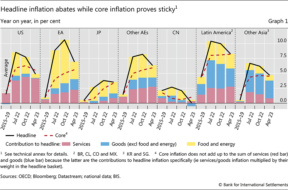
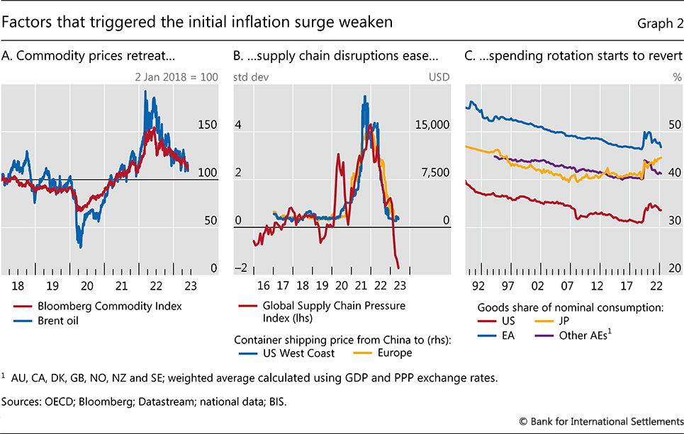
A longer-lasting amelioration came from easing global supply chain pressures, which largely normalised, allowing backlogs to be cleared (Graph 2.B). This affected primarily the prices of goods, which are much more heavily traded than services. These prices tended to rise more slowly and, in some cases, actually fell (blue bars in Graph 1). The pressure on goods prices was also eased by the ongoing reversion of the pandemic-related shift in consumption patterns away from services to goods (Graph 2.C).
That same rotation, however, boosted services price growth, which continued to rise (red bars in Graph 1). In the United States, the services component once again became the main factor behind inflation. Its contribution also slowly rose in other advanced economies (AEs) and in Latin America.
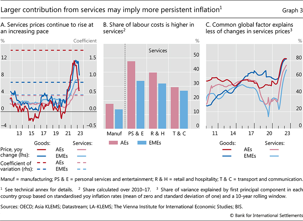
This shift in drivers of inflation towards services is likely to increase its persistence. The rate of change in services prices has historically been much less volatile than that for goods (dotted lines in Graph 3.A). Part of the explanation is that the share of labour in total costs in services is about twice as large as in manufacturing (Graph 3.B). This tightens the link between prices and wages. Not only are wage increases in general more inertial than other cost components, but they also tend to be more domestically driven in services, as the sector is less exposed to international competition. Indeed, the fraction of the variance of price changes explained by a global common factor has generally been lower for services, although it has risen recently owing to the widespread nature of the inflation surge (Graph 3.C).
Synchronised monetary tightening ends low-for-long
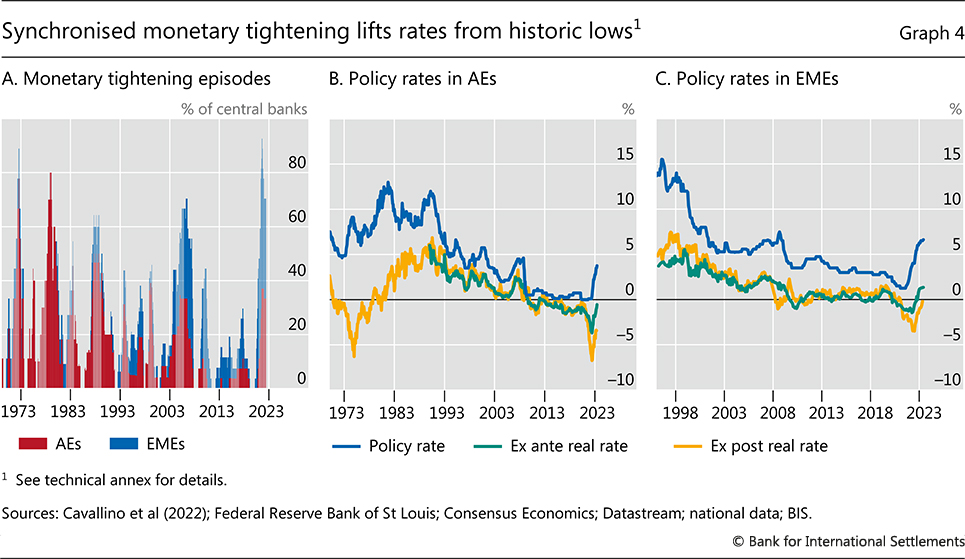
The inflation surge has led to the most synchronised and intense monetary policy tightening in decades.2 Almost 95% of central banks hiked their policy rates between early 2021 and mid-2023 (Graph 4.A). Historically, this share has rarely exceeded 50%, surpassing 80% only during the oil price shocks of the 1970s. Emerging market economy (EME) central banks raised policy rates at twice the historical pace, and AE central banks at a roughly similar one.3 4 Even so, policy rates are still below inflation and, in some AEs below inflation expectations, implying negative real rates (Graph 4.B and 4.C). At the same time, major AE central banks started to gradually shrink their balance sheets, with Japan as the exception. Quantitative easing turned into quantitative tightening.
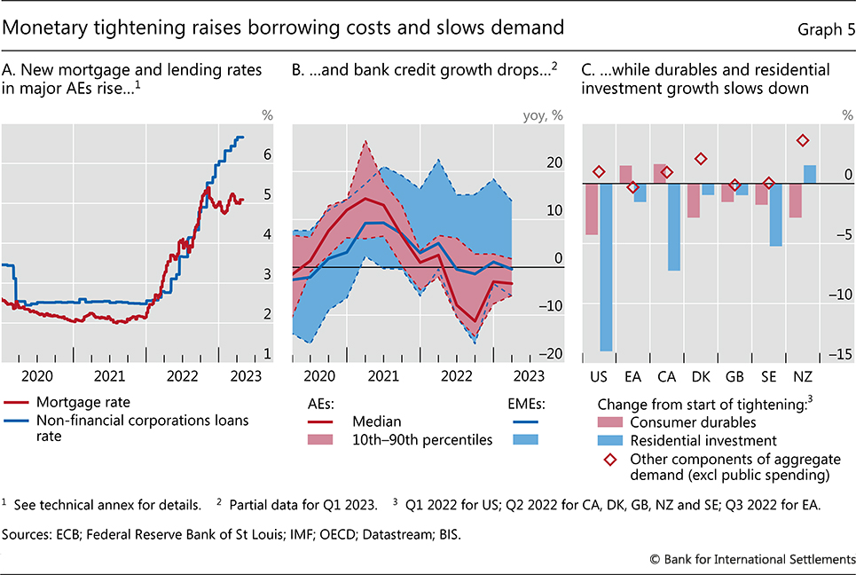
The transmission of monetary tightening to lending rates was mostly swift and began to weigh on aggregate demand. Borrowing costs rose for corporates and households alike (Graph 5.A). Bank lending standards tightened and bank credit contracted, especially in AEs (Graph 5.B). Consequently, spending weakened. The deceleration was led by the most interest rate-sensitive components of expenditure, such as consumer durables, and the housing market cooled in many economies (Graph 5.C).
The economy slows, but manages to avoid recession so far
Overall, global growth slowed from 6.3% in 2021 to 3.4% in 2022, weakening further in the first quarter of 2023 (Graph 6.A). The slowdown was most pronounced in AEs, from 5.7 to 2.8%. EMEs fared better, still growing at 4% in 2022 as a whole compared with 7.3% in the previous year. This was despite China recording a growth rate of only 3%, reflecting setbacks from large Covid-19 outbreaks and the drag from the real estate sector.
Still, activity held up better than expected in a number of key jurisdictions, and the much feared global recession did not materialise. Relative to the forecasts made early in the review year, growth outcomes in 2022 surprised on the upside in the United States, the euro area and most EMEs, with China an exception to the pattern. As high-frequency indicators remained robust in many jurisdictions, growth forecasts for 2023 were revised upwards as the new year started, although the consensus still saw a considerable slowdown for the year as a whole, to 2.6%.
The relative strength of economic activity and the upgrade of expectations for 2023 reflected three main factors.
Graph 6
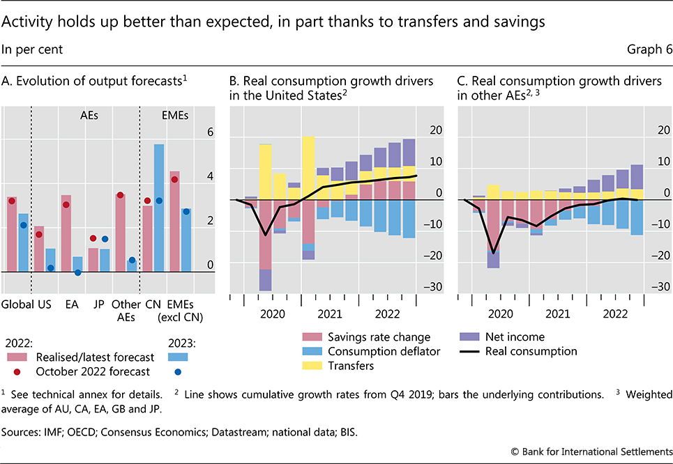
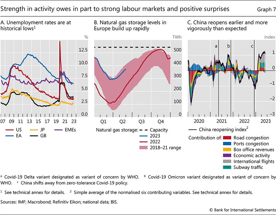
First, consumption remained robust. Excess savings accumulated during the pandemic, not least thanks to higher saving rates and fiscal support (red and yellow bars, respectively, in Graphs 6.B and 6.C). Once Covid-related restrictions were lifted, households drastically cut their saving rates, to pre-Covid levels in most AEs and to even lower ones in the United States. Further, buoyant labour markets bolstered income (purple bars in Graphs 6.B and 6.C). Unemployment rates fell to multidecade lows, especially in AEs (Graph 7.A). Job creation was strong in both AEs and EMEs while job vacancy rates remained high, around record levels in the United States and Europe.
Second, the energy crisis proved far less consequential than expected. A relatively mild winter and the rapid build-up of gas storage helped prevent the deep and widely forecast recession in Europe (Graph 7.B).5 And, in many jurisdictions, fiscal support insulated households and firms from the impact of higher energy prices.
Third, the rapid reopening of the Chinese economy in January, after the country abandoned its zero-Covid strategy in December 2022, boosted domestic activity (Graph 7.C). This also lifted activity abroad, although to a lesser extent than in the past, given the services-driven nature of the rebound (Box A).
Financial system shaken by bank failures
Financial markets and the financial system more generally started to adapt to the abrupt end of low-for-long interest rates but the process was far from smooth. A broad disconnect emerged between financial market pricing and central banks’ announced policy path. And rising signs of stress appeared in the financial system.
Box A
Spillovers from China’s reopening
China abandoned its dynamic zero-Covid policy in late 2022, starting to relax pandemic restrictions in November and reopening its borders in early January 2023. The timing and pace of reopening surprised the market, whose consensus as of early November 2022 was for a gradual reopening from March 2023.
After the reopening, the Chinese economy rebounded strongly, driven mainly by services. The Q1 2023 GDP advanced 4.5% year on year (Graph A1.A), topping the market consensus. Growth forecasts for 2023 were revised up from 4.5% in November 2022 to 5.8% in May 2023. The services sector (eg catering and tourism) benefited most from improved mobility, and the non-manufacturing PMI in March 2023 reached its highest level in more than a decade. The manufacturing sector started to recover from June 2022, after supply chain pressures eased, but faces headwinds in 2023, as external demand flags. Recovery in the construction sector is also likely to be modest, given weak sentiment in the real estate market.
Growth spillovers to the rest of the world from a services-driven recovery should be limited, because services are less tradable and more oriented towards domestic demand. This contrasts with construction and manufacturing, which require imports of raw materials and intermediate goods from other countries. Growth in construction and manufacturing in China had significant positive effects on other emerging market economy (EME) exports between 2004 and 2019 (Graph A1.B). For example, a 1% quarterly growth in construction activity increased exports to China from Asian manufacturing exporters by 0.7%, and those from Latin American metal exporters by 0.5% on average for the first four quarters, while a 1% growth in manufacturing output increased Asian exports to China by 0.6%. In contrast, services had no significant impact.
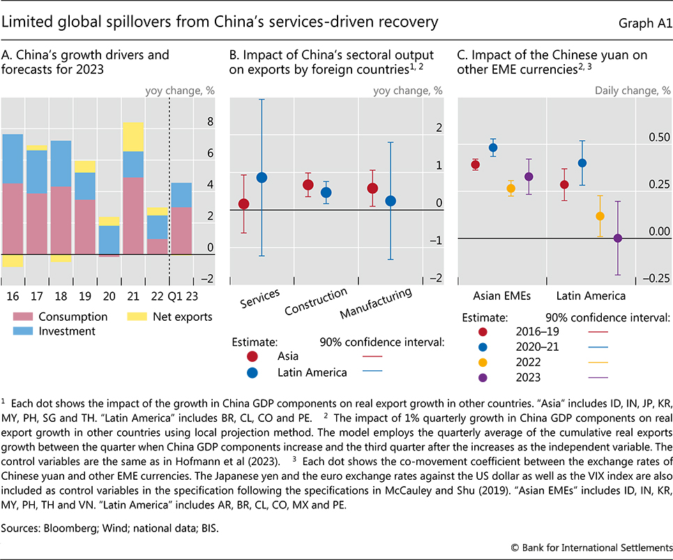
The spillover to global inflation could be small as well. One important channel through which China’s growth can affect global inflation is commodity prices. In particular, a pickup in manufacturing and construction activity in China would increase demand for commodities (metals in particular for construction), boosting their prices. Indeed, in 2004–19, a 1% increase in manufacturing production raised broad commodity prices by 2.2% after two quarters, while a 1% increase in construction activity raised metal prices by 0.9%. Again, services had no impact.
Consistent with a smaller spillover from China’s recovery this time around, financial assets in EMEs showed weaker co-movement with those in China in 2023 than in previous years. For example, the currencies of Asian and Latin American EMEs used to show strong co-movements with the Chinese yuan (Graph A1.C, red and blue dots). However, the co-movement weakened in 2022 when China diverged from some other parts of the world in terms of pandemic policy, the growth path and the monetary policy stance (yellow dots). The correlation remained at low levels for Latin America until May 2023, consistent with the expectation of limited spillover (purple dots). The co-movements of equity market returns and those of portfolio capital flows also diminished.
The eight Asian manufacturing exporters are India, Indonesia, Japan, Korea, Malaysia, the Philippines, Singapore and Thailand. The four Latin American metal exporters are Brazil, Chile, Colombia and Peru. Consistent with the dependence of spillovers on growth drivers, China’s spillover to the rest of world has varied over time. In particular, a 1% increase in China’s GDP was associated with 0.4% GDP growth in the rest of world in 2004–08 (when China actively participated in global trade after its entry into WTO in 2001), with 0.6% growth in 2009–14 (when China introduced large-scale investment projects after the 2007–09 Great Financial Crisis), and with 0.1% growth in 2015–19 (when China reduced reliance on investment for growth but focused more on consumption). The correlation between China’s equity market returns and those in Asian and Latin American EMEs was relatively high at 0.34 in 2016–19 and 0.36 in 2020–21 but fell to 0.17 in 2022 and Q1 2023. In contrast, the correlation of bond market returns stayed around zero throughout these periods. Similarly, after controlling for economic fundamentals, a one standard deviation increase in daily portfolio capital flows to China was associated with an increase in portfolio capital flows to six Asian EMEs and one Latin American country by 0.11 and 0.13 standard deviations in 2016–19 and in 2020–21, respectively, but its impact declined to 0.09 standard deviations in 2022 and Q1 2023.
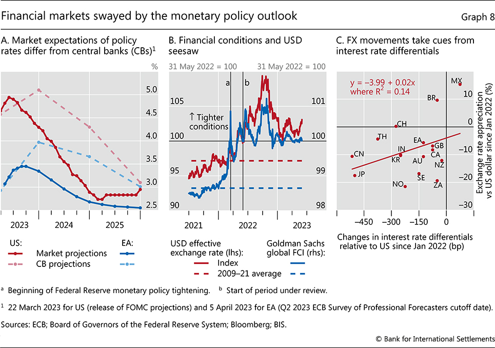
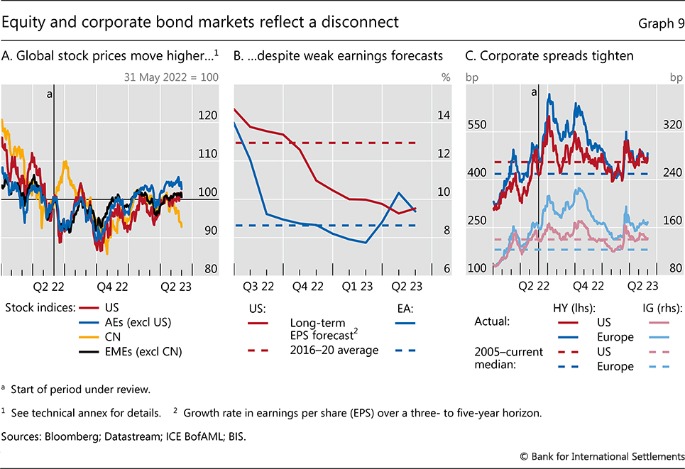
The disconnect between market expectations and central bank plans was evident in the dynamics of financial conditions. As markets were swayed by the shifting odds of inflation staying high and the economy entering a recession, participants continuously re-evaluated how central bank actions would evolve. Expectations of future rates remained lower than central banks’ projections, with investors anticipating rate cuts already in 2023 (Graph 8.A). After considerable tightening in 2022, by some measures, financial conditions tightened marginally during the period under review (Graph 8.B). They remained tighter than historical averages.
Foreign exchange movements largely followed those of financial conditions, taking their cue from the relative strength of the economies and the corresponding monetary policy outlooks. The US dollar generally appreciated through the third quarter of 2022, before weakening moderately against most currencies. By and large, the depreciation against the dollar was larger for the currencies of countries where the policy rate increased less than in the United States. The Japanese yen and the euro touched multidecade lows. Countries where monetary tightening had started earlier and interest rates had reached higher levels, such as Mexico and Brazil, actually saw appreciations (Graph 8.C). In general, EMEs absorbed the sharp tightening of global monetary conditions in an orderly way.
The disconnect between financial market expectations and central bank communications was also evident from the dynamics of risky assets. Equity markets finished the review period marginally higher (Graph 9.A), despite weak earnings forecasts, especially in the United States (Graph 9.B). Measures of implied equity volatility hovered below historical averages for most of 2023. In credit markets, spreads marginally tightened, remaining in line with historical norms in the United States and somewhat above in Europe (Graph 9.C).
Against this backdrop, increasing signs of stress emerged in the financial system in late 2022 and early 2023, in large part due to higher interest rates.
First, leveraged strategies to hedge against drops in interest rates came under pressure. As the UK “mini-budget” announcement in September 2022 sent gilt rates soaring, such strategies generated losses for the so-called liability-driven investment (LDI) funds in which UK pension funds had invested. To meet the ensuing collateral calls, LDI funds needed cash infusions, which pension funds failed to provide promptly enough. As their solvency positions worsened, LDI funds had to deleverage by selling gilts, putting further upward pressure on yields and setting off a full-fledged spiral. The Bank of England intervened forcefully and swiftly through temporary asset purchases to calm the market.
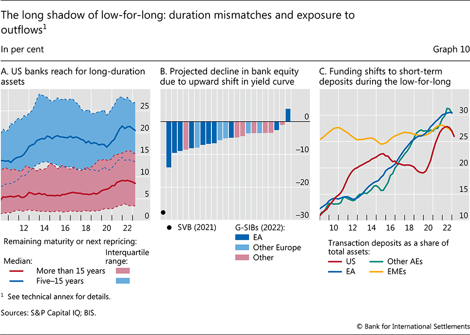
The sharp increase in interest rates also put the spotlight on banks. To the extent that they could reprice their assets, banks benefited from the impact of rising interest rates on net interest margins (Box B). However, during the low-for-long era, many had accumulated fixed rate mortgages and long-term government bonds (Graph 10.A), which declined steeply in market value when interest rates rose. Banks are generally required to assess and manage their exposure to changes in interest rates, including under scenarios of upward shifts in the yield curve (Graph 10.B). In addition to hedging with derivatives, banks often base their interest rate risk management on deposit stickiness. This feature has traditionally allowed banks to keep their funding costs in check by passing only a fraction of policy rate rises to deposit rates. As the share of short-term – and thus potentially flighty – deposits has risen (Graph 10.C),6 an increase in their interest rate sensitivity undermined the risk management strategies of some banks.
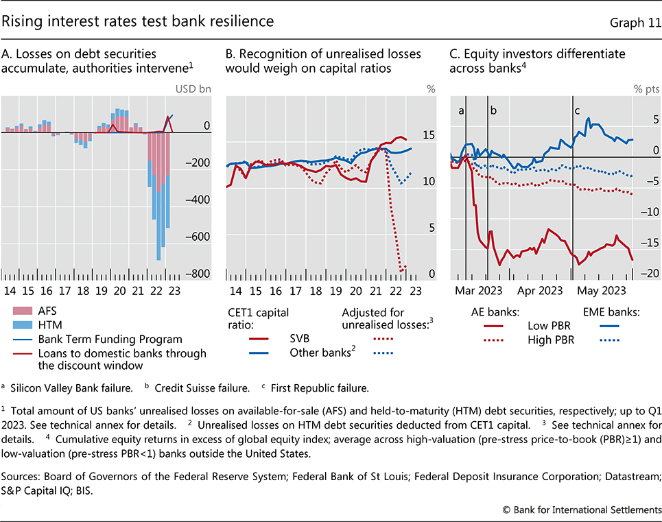
Mismanagement of interest rate risk, among other factors, drove the first major bank failures since the Great Financial Crisis (GFC). Already by late 2022, many US banks had sizeable market value losses on their debt securities holdings (Graph 11.A). More than half of the losses were not reflected on balance sheets, on the accounting assumption that banks would hold the attendant assets to maturity.7 However, as a loss of confidence in some of the smaller and thus more lightly regulated banks triggered a deposit flight, these banks had to liquidate some of their “held-to-maturity” assets and recognise immediate capital losses (Graph 11.B). These intertwined interest rate and run risks materialised forcefully for Silicon Valley Bank (SVB), a regional bank that collapsed in early March (Box C).
Box B
Rising policy rates and the outlook for banks’ net interest margins
While monetary tightening has exposed banks’ interest rate risk, the end of the low-for-long era is also expected to ease pressures on their income. In assessing banks’ performance, valuation losses on fixed rate assets will need to be set against higher interest income on variable rate assets and new lending. Drawing on evidence from past tightening episodes, this box assesses the effect of the recent rises in policy rates on net interest margins (NIMs), ie the difference between the yield on banks’ interest-earning assets and the cost of funding their debt.
During the current cycle, there was a general increase in NIMs (Graph B1.A). Since the start of the current cycle, NIMs have increased by more than 10 basis points in EMEs and nearly 5 basis points in AEs for every 100 basis point increase in the respective policy rate.
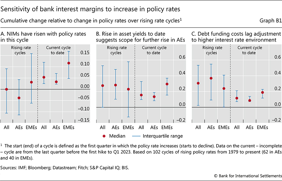
The recent rise in NIMs was driven more by the muted response in banks’ cost of debt than by the return on interest-bearing assets. In EMEs where the current cycle is more advanced, yields on interest-earning assets increased in line with past cycles, whereas the adjustment in debt funding costs is still lagging behind. The pickup in yields in AEs, by comparison, has yet to fully unfold if compared with the endpoint in previous cycles (Graph B1.B). This is consistent with banks’ shift to long-duration assets during the low-for-long era, which reduced the responsiveness of interest income to changes in policy rates. The increase in banks’ cost of debt, by contrast, has remained far behind historical endpoints (Graph B1.C). This probably stemmed from the higher proportion of non-interest-bearing deposits in many AE banking sectors.
The outlook for NIMs depends on how yields and costs will adjust to the policy path. Historically, NIMs often returned to their initial level, or even fell slightly in AEs, over the course of a rising rate cycle (Graph B1.A). At the current juncture, banks are expected to benefit from additional increases in yields when low-yielding fixed rate loans and mortgages expire, and borrowers refinance at higher rates. However, the availability of higher-yielding investments could also put upward pressure on bank funding costs. Relative to past episodes, this effect could unfold more rapidly due to the larger share of overnight deposits that can be withdrawn quickly. The threat of such withdrawals would require banks to pass on the increase in policy rates more swiftly to creditors in order to secure funding.
Return on interest-earning assets is defined as banks’ gross interest income divided by total interest-earning assets. Cost of funding is defined as banks’ interest expenses divided by total funding.
Box C
Recent bank failures
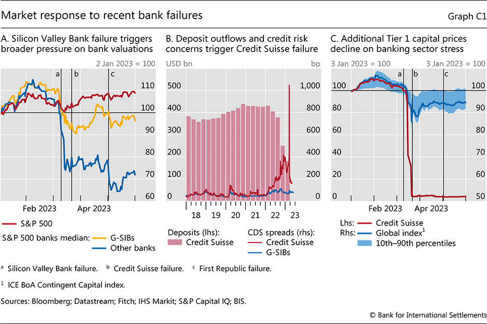
Market tremors in March 2023 highlighted how risk management deficiencies at individual banks can undermine the confidence of depositors and other investors, leading to a funding crisis that can reverberate through the financial system. This box reviews recent bank failures and attendant market responses.
Silicon Valley Bank (SVB), which was the 16th largest US bank as measured by total domestic assets at end-2022, went into receivership on 10 March 2023. SVB had accumulated significant, albeit unrealised, valuation losses on its unhedged securities portfolio due to rising rates over the course of 2022. In early March, confronted with persistent deposit outflows, the bank had to sell securities and recognise a large loss and the attendant impact on its capital position. Unable to raise new equity to rebuild this position, the bank collapsed within just a few days on the back of a concerted, unprecedentedly fast run by its mostly uninsured corporate depositors.
Following the failure, concerns spread immediately about similar vulnerabilities at other banks, leading to significant falls in the valuations of small and mid-sized banks amid large deposit outflows (Graph C1.A). After suffering a run by uninsured depositors, Signature Bank was closed two days after SVB’s failure. First Republic, also struggling with a combination of losses on long-duration assets and large deposit outflows, initially managed to secure alternative funding, including from major US banks. However, the bank ultimately failed given the persistence and scale of deposit outflows and, after entering receivership, was sold to JPMorgan Chase.
Concerns also spilled over to banks outside the United States. In particular, Credit Suisse entered the eye of the storm. This bank’s profitability and reputation had already suffered due to risk management deficiencies and significant performance setbacks in recent years. Market scepticism about the bank worsened through 2022 amid large deposit withdrawals, rising credit spreads and outflows of assets under management. The switch to a risk-off environment in March 2023 was the tipping point, with the bank’s CDS spreads jumping to levels indicating imminent default (Graph C1.B). To alleviate systemic risk concerns, Swiss authorities facilitated and enforced a takeover by UBS.
The Credit Suisse takeover shook the market for Additional Tier 1 (AT1) capital – instruments that can be written down or converted to equity when a bank becomes unviable. As the takeover entailed the writedown of Credit Suisse’s entire AT1 capital, this led to broader uncertainty about when and how these instruments would absorb losses at failing banks. The immediate upshot was significant price declines in the AT1 market, notably for instruments issued by European banks (Graph C1.C). New issuance on this market has been subdued, even if prices have since partially recovered after European authorities provided additional clarity on the hierarchy of AT1 investors relative to equity holders in the event of bank failure.
Graph 10
The realisation of interest rate risk reverberated through the US banking sector in the first half of 2023. Small and mid-sized banks suffered significant deposit outflows, forcing the closure of first Signature Bank and then First Republic Bank. At the same time, US global systemically important banks (G-SIBs) saw significant inflows from depositors searching for safe havens.
Investors’ concerns spread to banking sectors in several other AEs. Banks that had already faced persistent market scepticism, as indicated by a low price-to-book ratio (PBR), were hit particularly hard. Credit Suisse – a G-SIB which had been struggling with large fund outflows and a series of setbacks (see Box C) – failed to rebuild market trust and – after writing down its contingent convertible bonds to absorb losses – was taken over by a competitor. Relative to global equity markets, other AE banks with low PBRs also registered deeply negative stock returns (Graph 11.C). This stood in contrast to the more modest decline for high-PBR banks in AEs and banks in EMEs.
Again, authorities responded forcefully to contain contagion and deployed a number of crisis management tools to curb systemic risks. In the United States, authorities invoked the so-called systemic risk exception – previously used in the GFC – to stem more widespread runs by guaranteeing the uninsured deposits of SVB and Signature Bank. In addition, the Federal Reserve established the Bank Term Funding Program (BTFP), offering loans to banks that pledged qualifying government securities, valued at par and thus above market value. The BTFP complemented lending through the Federal Reserve’s discount window, which soared in the immediate aftermath of SVB’s failure but has come down since then (Graph 11.A). In Switzerland, the public sector backed the emergency takeover of Credit Suisse, with the central bank pledging significant liquidity support and the government extending guarantees to shield the central bank from potential losses. Furthermore, to facilitate the takeover, the government guaranteed to cover part of future losses in relation to the disposal of the failed bank’s legacy assets.
Key risks on a turbulent path
Against this broad macroeconomic and financial backdrop, what is the outlook for the global economy?
Consensus forecasts are rather benign. While forecasters do see lower growth and inflation still above target, the slowdown is rather mild and the fall in inflation substantial. Banking woes are expected to be contained.
Two risks loom large, however – quite apart from those of a more political nature, such as an intensification of geopolitical tensions. First, disinflation could well turn out to be harder than expected – the “last mile” challenge. Second, the end of low-for-long could further test the global financial system, with the crystallisation of macro-financial risks to threaten growth.
This combination of risks is rather unique by post-World War II standards. It is the first time that, across much of the world, a surge in inflation has coexisted with widespread financial vulnerabilities. The longer the inflation persists, the stronger and longer the required policy tightening, and hence the bigger the financial stability risks.
The “last mile” may pose the biggest challenge
Getting back to target is likely to be harder than the first phase of the disinflation journey. There are several reasons why. Beyond fading base effects and the increasing role of inertial components of inflation, households and firms may adjust to persistently higher inflation by trying to recoup previous losses and then seeking to avoid future expected ones through their wage- and price-setting decisions.8 Moreover, as time goes by and higher policy rates propagate through the system, the economy will weaken and further financial stress may arise. This means less pressure on prices but, at the same time, tougher trade-offs involving activity. In some cases, there may be political pressure on central banks to keep interest rates low, requiring them to reiterate the commitment to deliver price stability through both communication and action. Such dynamics may be especially relevant among those EMEs where institutional safeguards are weaker, inflation expectations are less anchored and indexation is more prevalent.
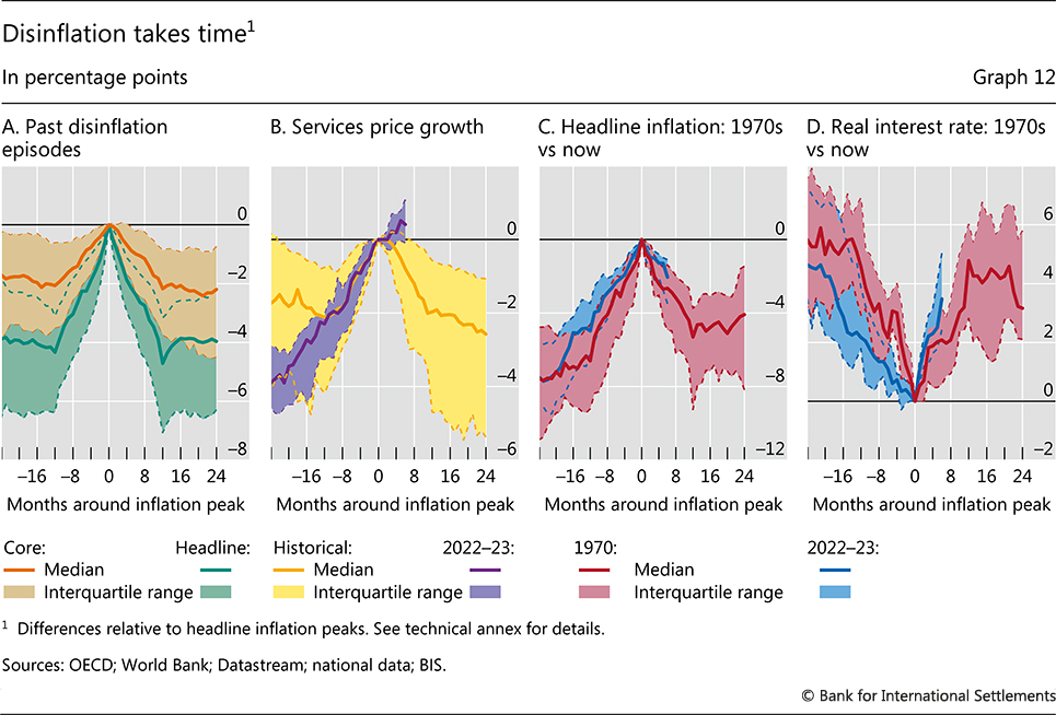
Admittedly, in previous disinflation episodes, headline inflation typically returned to the pre-peak levels (or even lower) in the space of one to two years (Graph 12.A). Core inflation tended to follow a similar path.
However, a number of features set the current episode apart from previous ones and indicate that disinflation may prove difficult. First, services prices have risen much faster and their rate of change has not yet peaked (Chart 12.B). This could mean a potentially longer disinflation journey. Second, rather than the median episode, the current surge more closely resembles the 1970s – when a “first mile” of disinflation was achieved in the space of about one year but inflation thereafter declined only gradually: after two years, it was still generally above its pre-surge level (Graph 12.C). In fact, the pace of disinflation so far has been even slower than in the 1970s – although the tightening has proceeded at a faster pace (Graph 12.D).
Crucially, then, what is the likelihood of a transition to a high-inflation regime, such as the one in the 1970s?
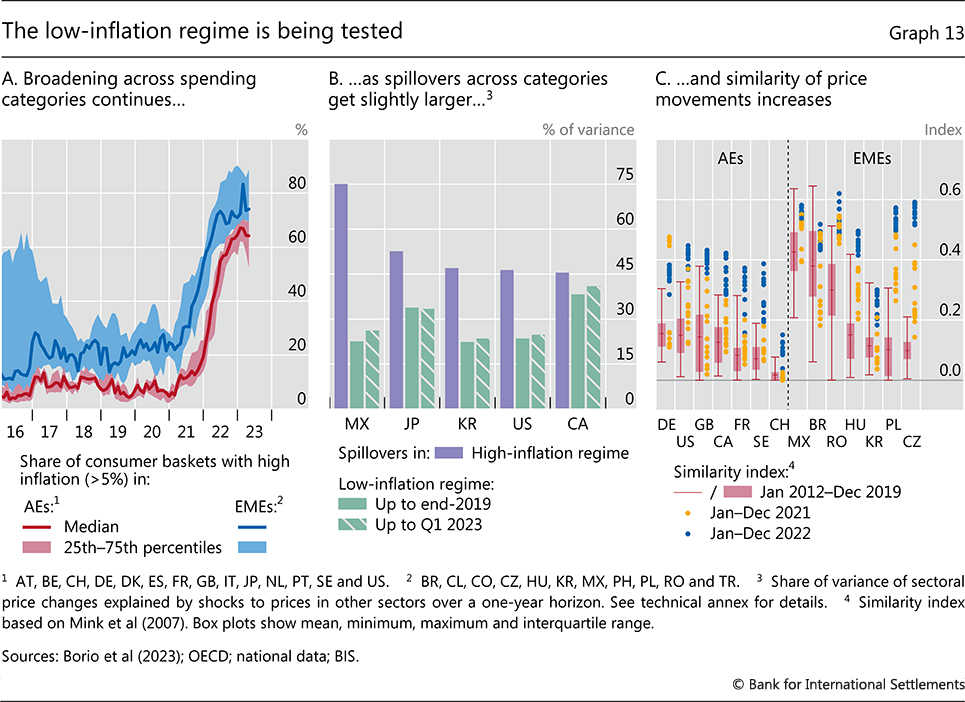
Several indicators point to possible obstacles along the disinflation journey and suggest that the low-inflation regime will continue to be tested. First, after a steep rise, the share of items in the consumer price index whose prices increased at a fast rate has not come down (Graph 13.A). Second, price spillovers across consumption categories are slightly larger than they were in the recent past when inflation was low (Graph 13.B). This means that increases in the price level due to price shocks in one category will propagate to others, raising the likelihood that they will lead to sustained inflation rather than die out. Third, price changes across categories are becoming increasingly similar (Graph 13.C), implying that differences in consumption patterns across consumers and input costs across firms matter relatively less, so that the general price level becomes more relevant for individual decisions. This tends to be a useful indicator of inflation persistence, ie when the similarity index is high, so is the probability that inflation in the next period will be at least as high as in the current one.9 These signals, taken together, suggest that households and firms are responding more strongly to the higher inflation rates.
Looking ahead, two closely related factors could signal a shift in inflation norms and tip the disinflation process off course: self-sustaining wage-price dynamics and a de-anchoring of inflation expectations.
While nominal wage growth has not been exceptionally strong so far, this should not provide too much comfort. Wage adjustments are still influenced by the lingering effects of the norms prevalent in the low-inflation regime, but this could change quickly. The inflation surge has severely eroded the purchasing power of households (Graph 14.A), even more than in past disinflation episodes (Graph 14.B). Some catch-up is on the cards, particularly given the strength of labour markets. While labour’s bargaining power declined significantly over the years of low inflation,10 recent strikes and calls for unionisation suggest that the environment is evolving. In the euro area, for instance, negotiated wage growth has been on the rise and is now at its highest level since the inception of the common currency. And while multi-year wage contracts generally make the adjustment lags for wages considerably longer than for prices, contract length may shorten in response to higher and more persistent inflation.11 What’s more, the pass-through from prices to wages has been somewhat higher when labour markets have been tight.
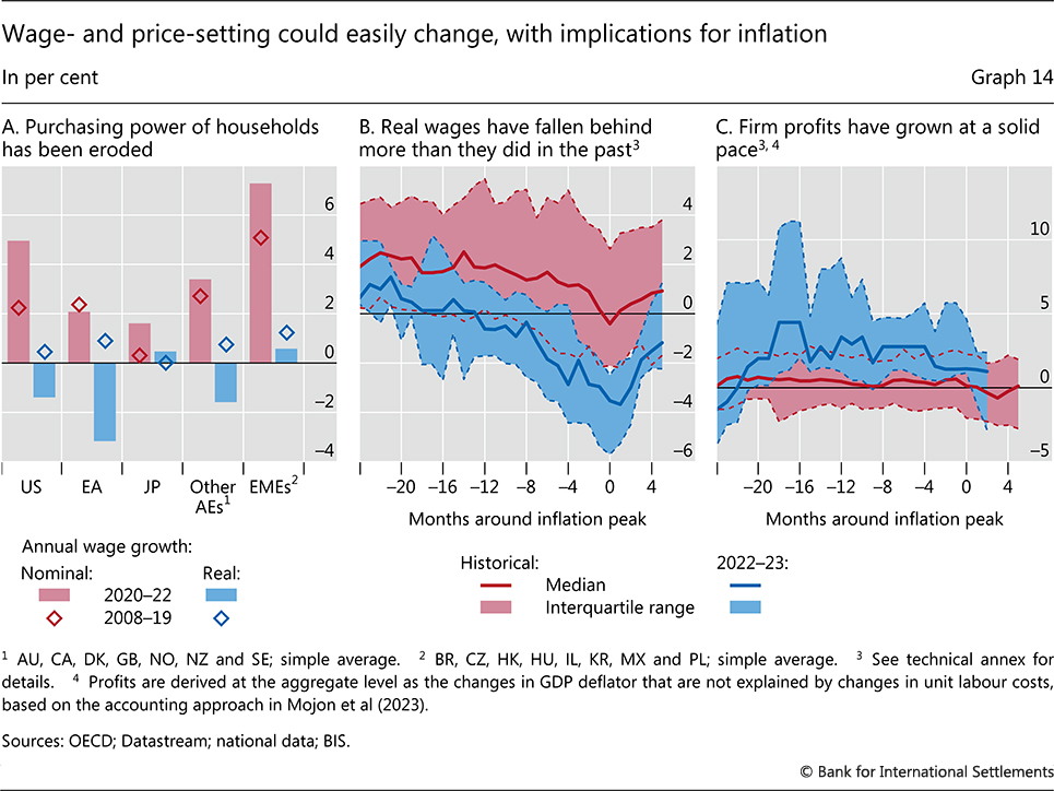
In parallel, there are signs that price-setting behaviour is changing. Firms are adjusting prices more frequently than when inflation was low and stable.12 In addition, corporate profits, which were already on the rise before the inflation surge, have held up remarkably well so far (Graph 14.C). This is a departure from the historical pattern: in past episodes, profit growth tended to fluctuate within a comparatively narrow range around zero. One concern is that, having been able to raise prices more easily than in the low-inflation regime, firms are now more reluctant to accept profit squeezes and will pass on cost pressures to prices more readily.13
In the end, a shift to a high-inflation regime would require self-sustaining wage-price increases – a “wage-price spiral” – as workers and firms try to recoup their losses. The feedback between wages and prices has been quite low in the last two decades, below 10%. However, moving to a high-inflation regime would strengthen it.14
A stylised exercise based on a decomposition of changes in the GDP deflator during disinflations shows that some catch-up in wages would be compatible with inflation returning to target, but only as long as firms accept a reduction in profits.15 16 Back-of-the-envelope calculations suggest that, for inflation to go back to a target of 2%, profits on average would need to decline by about 2.5% per year in 2023–24, should real wages rise fast enough to make up for the loss in purchasing power and return to the pre-inflation surge level by end-2025. For comparison, the cross-country pre-pandemic median for profit growth has been slightly more than 1.5% between 2014 and 2019.17
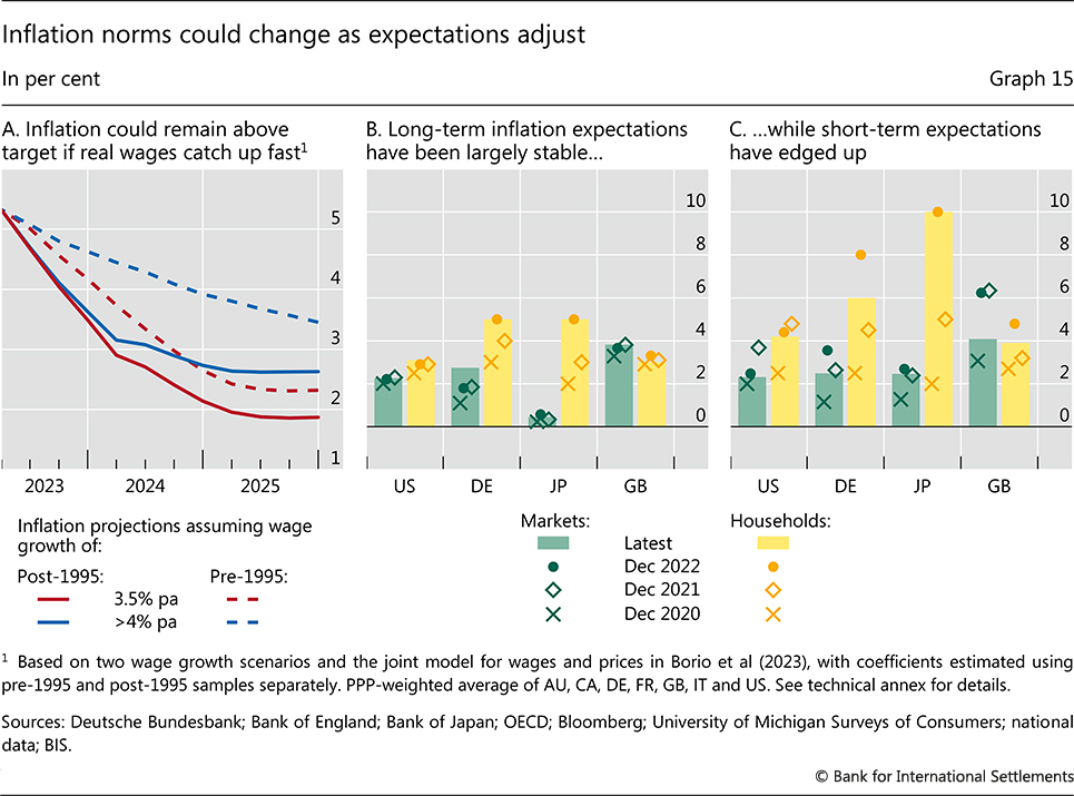
An alternative exercise based on the historical price-wage relationship reinforces the message that the room for adjustment in real wages without jeopardising the inflation target is limited. The exercise is guided by the cointegration between core CPI and hourly compensation and considers the path inflation could take under two different scenarios of purchasing power recovery (Graph 15.A).18 In the first scenario, wages gradually recover, growing at an annual rate of 3.5%, which is consistent with an inflation target of 2% and historical labour productivity growth rate of 1.5% (“gradual catch-up”). Real wages would then largely make up for the losses incurred so far by end-2025. In the second one, the pace of nominal wage growth is faster in 2023 and 2024 at 6%, and settles at 4% by 2025 (“fast catch-up”). In that case, the erosion in real wages is remedied by mid-2024. The gradual catch-up scenario seems conducive to bringing inflation down to or below target (solid red line in Graph 15.A), based on the historical relationship between wages and prices that prevailed in a low-inflation environment – here proxied by post-1995. By contrast, inflation would remain well above target up to the end of 2025 in the fast catch-up scenario (solid blue line in Graph 15.A). Further, if the relationship between wages and prices reverts to the pattern that prevailed before 1995 – capturing a high-inflation environment – the implied inflation trajectory would remain above target also in the gradual catch-up scenario (dashed red line in Graph 15.A). This is because wage-price spillovers were stronger when inflation was higher.
A wage-price spiral would be even more likely should workers and firms seek not just to recoup past losses, but also to be compensated for future ones, ie if expectations became “de-anchored”. While a de-anchoring is not yet evident, inflation expectations have edged up visibly in some cases and are generally above target. True, long-term ones – over a five-year horizon – have remained stable. That said, they are higher than before the inflation surge began. This is especially so for German and Japanese households, who had seen inflation being persistently below target before the pandemic (Graph 15.B). Further, short-term inflation expectations – at the one-year horizon – rose much more than their long-term counterparts (Graph 15.C). The longer inflation remains high, the higher the odds that long-term expectations will follow.
Macro-financial vulnerabilities could complicate the inflation fight
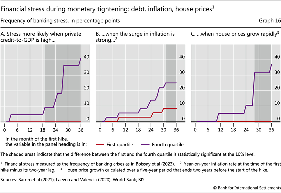
Given the economic background, the risk of further financial stress is material. Historically, about 15% of monetary policy tightening episodes are associated with severe banking stress. The frequency of such stress is higher during tightening episodes that start in an environment of high debt, an abrupt inflation surge or rapid house price growth. If the private debt-to-GDP ratio is in the top quartile of the historical distribution at the time of the first interest rate hike, 40% of the episodes are followed by a banking crisis within three years (Graph 16.A). The odds of a banking crisis are 25% for an inflation surge (Graph 16.B) and about 35% for rapid house price growth (Graph 16.C). Very high debt levels, a remarkable global inflation surge, and the strong pandemic-era increase in house prices19 check all these boxes. Vulnerabilities in the commercial real estate (CRE) sector – historically a common source of stress in the banking sector – raise concerns, too (Box D).
If inflation proves to be more persistent than expected and central banks have to tighten monetary policy by more or for longer, financial stability risks will rise. A key channel is the impact of asset prices and debt burdens on the macroeconomy. Sharply higher mortgage financing costs, coupled with high household debt (Graph 17.A) and falling house prices, translate into lower consumption (see Box D). Evidence shows that, generally speaking, high debt amplifies the impact of monetary tightening20 and that house prices are much more sensitive to a rate hike when debt levels are high.21 Countries with higher household debt have already seen a sharper rise in debt service ratios (DSRs) (Graph 17.B). Economies that rely on adjustable-rate mortgages (ARMs) are especially vulnerable (Graph 17.C).
Illustrative simulations, based on historical relationships, shed light on the implications of alternative interest rate paths. For a number of AEs, the simulations trace the behaviour of key variables in three scenarios, assuming that interest rates are constant, follow the “market path” or go “higher-for-longer”, ie remain at the market-implied peak plus 200 basis points until the end of 2027 (Graph 18.A). Average AE private sector DSRs could increase by about 1.5 percentage points and reach their pre-GFC peaks by 2027 if central bank policy rates evolve as financial markets currently expect (Graph 18.B). In the “higher-for-longer” scenario, average DSRs could increase by more than 4 percentage points. The decline in house prices in this adverse scenario could be as large as 30%, relative to the 15% drop in the market-implied path (Graph 18.C). The level of GDP in the adverse scenario could be about 2% lower by end-2027 relative to what would be expected were policy rates to follow the market path (comparing the blue to the yellow bar in Graph 18.D).
Box D
Commercial and residential real estate markets
This box first describes the trends in commercial real estate (CRE) markets, then discusses residential real estate (RRE) developments and concludes with an analysis of risks.
CRE dynamics
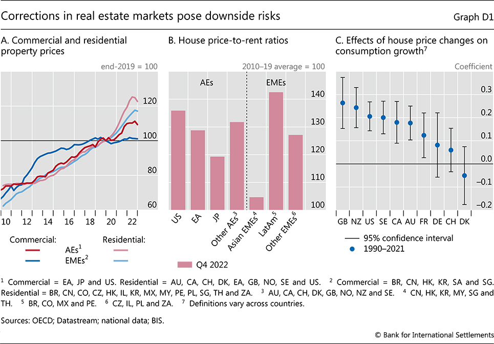
Commercial property markets weakened in emerging market economies (EMEs) during the review period (Graph D1.A). Following a brief period of robust gains, CRE prices in advanced economies (AEs) reached a plateau and dipped slightly. EMEs generally saw the trend of weak CRE prices continue, with sharp price declines in some cases (eg Singapore).
The weakness in commercial property markets reflects a combination of cyclical and structural factors. Higher interest rates played an important role. In addition, office real estate saw sustained pressure as pandemic-era work-from-home activity evolved into permanent remote and hybrid work practices (eg office vacancy rates in the United States stood at almost 20% in the first quarter of 2023, about 6 percentage points higher than in the last quarter of 2019). Retail real estate continued to face headwinds due to greater e-commerce activity.
RRE dynamics
Residential property prices in many economies softened considerably as interest rates climbed. During 2022, many AEs saw house price growth stall or even reverse direction. This weakness persisted into 2023 with only a few exceptions. Markets that had seen particularly strong price increases during the pandemic experienced some of the steepest drops (eg Australia and Canada). House prices also softened in many EMEs, although usually by less than in AEs (Graph D1.A). The gentler softening among EMEs mirrored the generally slower pace of price gains seen during the pandemic.
Valuations are still expensive by historical standards. Price-to-rent ratios have remained at very high levels in most AEs and EMEs (Graph D1.B). This points to further potential price drops.
Risks
The combination of falling house prices, high debt and rapidly rising debt service ratios is likely to increase the number of borrowers facing repayment difficulties for residential mortgages. While delinquency rates on residential mortgages are still low, they are expected to rise in some jurisdictions. For example, in January 2023, the UK Financial Conduct Authority warned that about 9% of UK mortgages are at risk of defaulting in 2023–24.
The downturn in RRE markets has already weighed on activity and a further, disorderly fall in house prices poses a major risk to economic growth. A fall in house prices could weigh on consumption growth due to negative household wealth effects, a reduction of pledgeable collateral and reduced consumer confidence. By some estimates, a 10% decline in house prices reduces (median) consumption growth in the following year by about 1.8% (Graph D1.C). The effect is strongest in countries with high home ownership rates, such as the United Kingdom and New Zealand, and is most pronounced where high home ownership is combined with a heavy reliance on adjustable rate mortgages.
Although smaller than RRE markets, CRE markets also raise a prominent risk to financial stability. Spreads on US commercial mortgage-backed securities (CMBS) rose substantially throughout much of 2022, reflecting a growing difficulty in refinancing maturing debt. In Sweden, where CRE firms rely heavily on bank funding and floating rate loans, a number of large property groups suffered from rating downgrades and stock sell-offs. CRE delinquencies started to pick up in some markets and global distressed CRE debt was close to $175 billion in early 2023, vastly more than in other sectors. CRE prices tend to be more sensitive to the business cycle than RRE prices and to react more strongly to a downturn. Moreover, the performance of banks has historically been sensitive to CRE price developments, raising the risk of a credit crunch. In addition to direct exposures to CRE, particularly in regional banks, some banks have large indirect exposures through other channels, eg via construction lending. Troubles with CRE lending can thus have an outsize impact on overall bank lending. Non-bank financial institutions and foreign investors are also important and growing providers of credit to the CRE sector. Their retrenchment could lead to sizeable asset fire sales, which could in turn destabilise financial markets, as seen during the recent episode of regional bank failures.
Bank vulnerabilities
Further illustrative simulations explore the possible implications for banks. Credit losses on the back of rising debt service ratios could undermine the support that banks receive from higher interest income. If macro-financial conditions follow the “market path” scenario, banks’ expected credit losses in 2025–27 would be close to the average level in AEs over the past three decades (Graph 19.A). In the “higher-for-longer” scenario, those losses could approach the levels seen during the GFC, subject to a large degree of uncertainty (Graph 19.B).
Losses in banks with large exposures to interest rate-sensitive sectors could be heavier. A prime example is the CRE sector, which faces additional risks from the post-pandemic reduction in demand due to hybrid work arrangements. Smaller and more regionally focused banks in many AEs tend to have a greater concentration of loans in this sector.
Low valuations and weak profitability go hand in hand, heightening banks’ vulnerability to losses. A number of GSIBs had persistently low PBRs throughout the low-for-long era. This is a sign of stubbornly sub-par profits and/or persistent investor scepticism about the bank’s ability to create value (Box E). Low profits weaken the first line of defence against losses. In addition, low PBRs limit a bank’s capacity to generate equity capital internally: shareholders prefer that profits be paid out rather than be reinvested at a lower return. When adjustments are necessary at short notice, however, banks may have to seek external capital. This can trigger adverse market responses, especially when investor confidence is fragile.
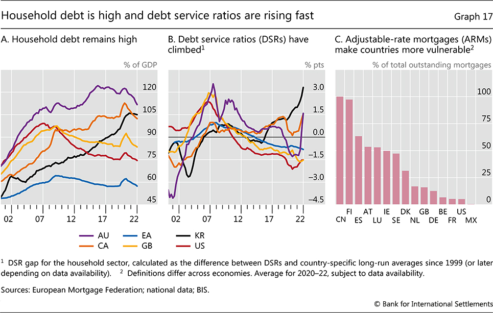
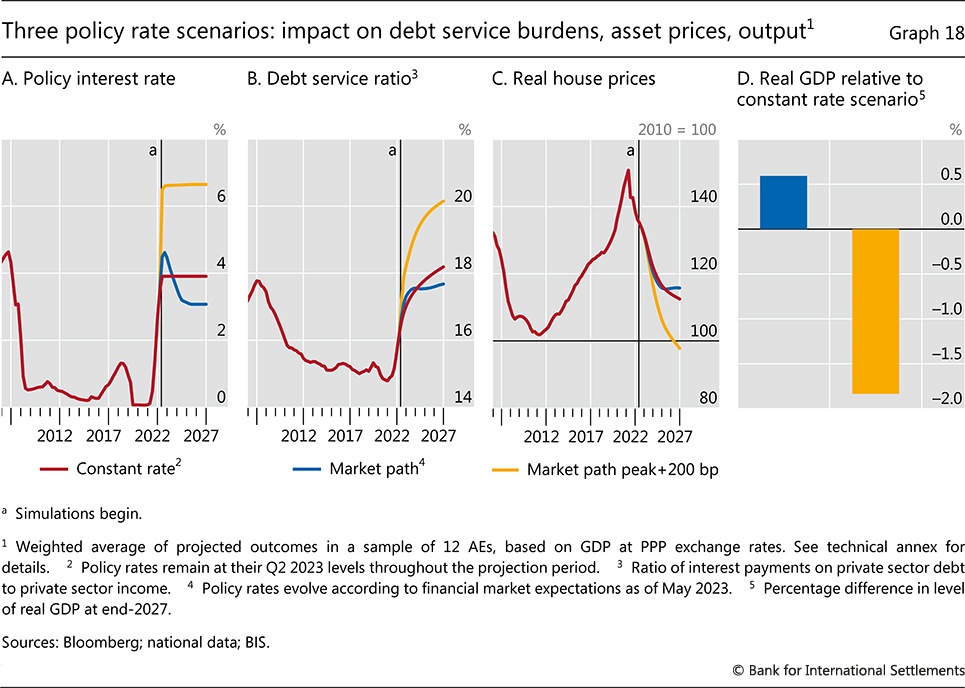
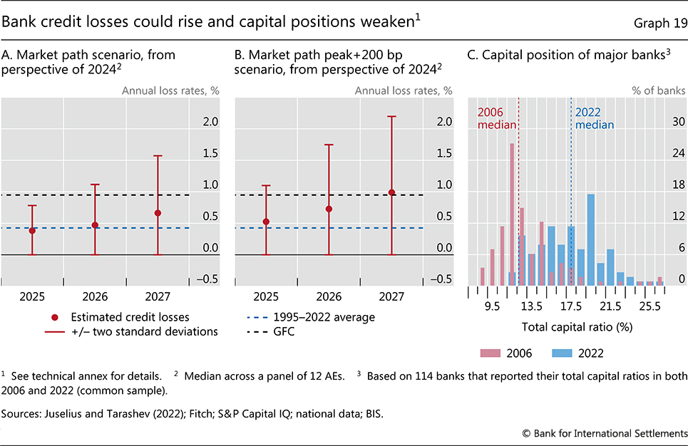
Post-GFC, financial reforms have greatly bolstered the capitalisation of the banking sector (Graph 19.C) and have encouraged more forward-looking loan loss provisioning. Ultimately, the impact on the banking sector will depend on the extent to which its loss-absorbing capacity helps preserve investor confidence.
Vulnerabilities among NBFIs
The long period of unusually low interest rates provided fertile ground for the build-up of widespread vulnerabilities in the NBFI sector. Moreover, post-GFC, this sector has grown in leaps and bounds relative to the banking sector.22 In the process, risks there have increased and some vulnerabilities have attained systemic importance. Not all of these vulnerabilities have been properly identified because large parts of the NBFI sector are quite opaque.
The NBFI sector can be a source or amplifier of systemic stress through several mechanisms. First, among NBFIs, hidden leverage and liquidity mismatches are rife. In addition, duration management by NBFIs – such as life insurance companies – could have adverse spillovers when a sharp rise in interest rates shortens liability duration and prompts sales of long-duration assets in a falling market. Stress could also stem from the interlinkages between NBFIs and banks via funding or hedging activities.
Vulnerabilities in two specific market segments deserve mention.
First, liquidity mismatches at investment funds can exacerbate existing fragilities in the real estate sector and corporate bond markets. An intensified downturn in real estate markets could, in particular, trigger large withdrawals by investors in REITs. In turn, this would require REITs to sell into inherently illiquid markets, setting in motion a downward price spiral. Similar liquidity mismatches could also affect corporate credit – a market segment that has seen a secular deterioration in credit quality, as reflected in the trend decline in ratings. In this case, large redemptions from bond mutual funds and ETFs could trigger fire sales.23
Box E
Structural challenges among global banks: hints from market valuations
The price-to-book ratio (PBR) reflects investor perceptions of a bank’s capacity to generate value. A number of global systemically important banks (G-SIBs) have PBRs considerably below unity – ie the market value of their equity has been persistently below the accounting, or book, value. Such low PBRs show that investors doubt the viability of these banks’ business models. This box reviews the drivers and policy implications of low PBRs.
Expectations of banks’ future profitability are a key driver of banks’ valuations. There is a tight relationship between a bank’s forecast return-on-equity (RoE) and its PBR (Graph E1.A). Over the past decade, three groups of G-SIBs have emerged: high-PBR banks that have convinced investors of their capacity to deliver strong profits, resulting in a PBR above 1; mid-PBR banks with market valuations close to, but below their book value; and low-PBR banks with persistent profitability challenges and hence low valuations.
Profitability differences notwithstanding, all banks need to generate sustainable returns for their shareholders. High- and mid-PBR banks have been able to satisfy shareholders by disbursing only a fraction of their profits in the form of dividends or share buybacks. By contrast, many low-PBR banks have had to pay out their entire profits, not least because reinvesting in an underperforming balance sheet does not appeal to shareholders. Indeed, this seems to have been necessary for low-PBR banks in order to put a floor under their share prices, given the tendency of valuations to adjust such that they deliver comparable dividend yields (Graph E1.B).
As low-valuation banks face challenging market conditions, they have become increasingly owned by public entities. Raising capital externally is particularly dilutive for the incumbent shareholders of such banks. This helps explain why equity investors most strongly punish these banks in the face of adverse results that may force these banks to tap markets for funds (Graph E1.C). In turn, such challenges are consistent with domestic and foreign governments purchasing more than 40% of the new equity issued by low-PBR G-SIBs from 2014 to 2022.
Graph E1
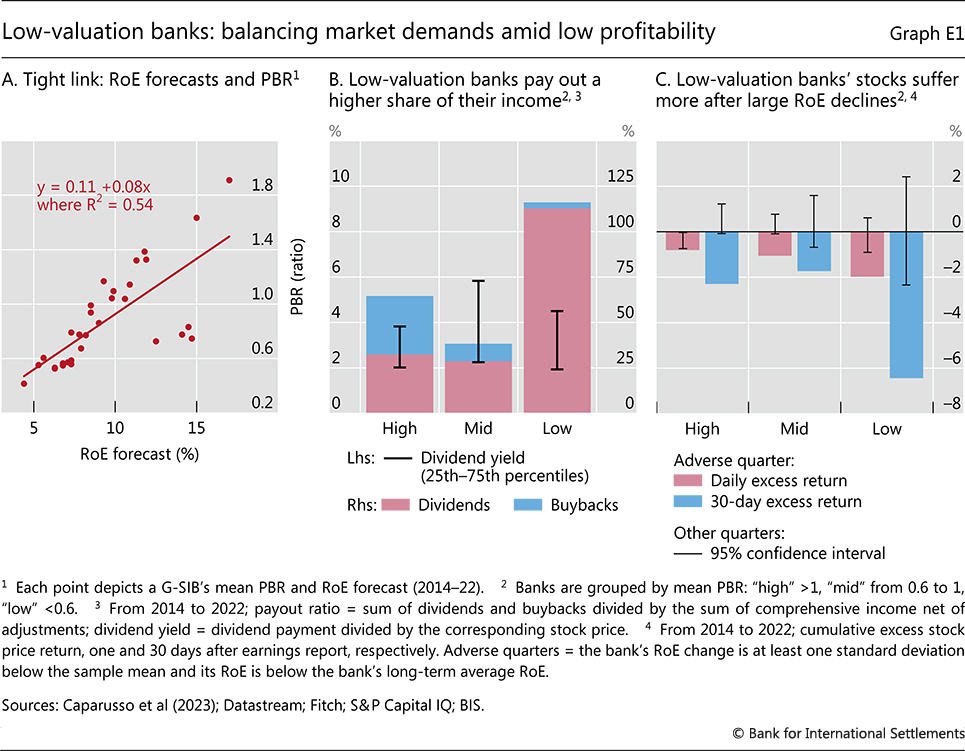
With profits distributed to meet shareholder expectations, low-valuation banks have had to reduce the riskiness of their assets in order to meet stringent capital requirements. This has surfaced, for instance, as retrenchment from trading or cross-border activities. In the near term, a retrenchment could temporarily impair financial conditions in specific segments. But, over the medium term, it should enhance the efficiency of financial intermediation by shifting the provision of financial services from less to more profitable business models.
Public authorities could facilitate the transition of low-valuation banks to more sustainable business models. For one, they could support banks in addressing legacy issues, removing impediments to cross-jurisdictional mergers and acquisitions, and providing incentives to raise investment in restructuring efforts. Banks with profitable business models play a vital role in underpinning market confidence and in providing reliable funding for the real economy.
For a more comprehensive review, also covering how banks’ response to stricter capital regulation has depended on their valuation, see Caparusso et al (2023). See, for example, the analysis in Goel et al (2021) or in Caparusso et al (2019).
Second, even though private equity and private credit funds take on minimal liquidity risk, their contribution to corporate indebtedness is a cause of concern. Private market deals grew more than fivefold after the GFC and reached a multidecade high of almost $500 billion globally at the end of 2021.24 The funds’ highly procyclical risk-taking contributed to the build-up of leverage during the low-for-long era,25 thus sowing the seeds for stress when interest rates rose.26 As borrowing costs increase, the highly leveraged companies that private funds have invested in could face difficulties in refinancing and repaying their debt, a large share of which is estimated to mature in the next three years. A deterioration of these borrowers’ ratings would amplify these difficulties. Debt restructuring for distressed companies could buy time but, in the case of flawed business models, default would be inevitable. Banks could then incur losses directly, since some of them reportedly still warehouse significant amounts of the leveraged loans provided during the 2021 boom in private market deals.
Additional considerations in EMEs
While EMEs have so far been spared from significant spillovers from the financial stress in AEs, this could change. EMEs’ resilience reflects a range of factors, such as early monetary policy tightening (notably in Latin America), implementation of structural reforms, less foreign currency borrowing and reduced foreign investor participation in local currency bond markets. Nevertheless, beyond the home-grown vulnerabilities in some EMEs, such as in real estate and corporate markets, financial stress in AEs could at some point spill over through several channels. The exchange rate continues to play a particularly important role in this context. Furthermore, while the lengthening of debt duration reduces EME borrowers’ rollover risk, it also increases investors’ market risk. It can thus be thought of as the duration equivalent of “original sin redux”, ie the shift of exchange rate exposures from borrowers to lenders.
Navigating from turbulence to safety
Policymakers are facing tough challenges in the near and longer term. In the near term, the overriding challenge is to bring inflation back to target in the context of heightened financial stability risks. This challenge contrasts with those faced from the 1970s up to the mid-1980s, when inflation generally rose against the backdrop of limited financial strains. Thereafter, financial stress broke out during generally quiescent inflation (Chapter II). The combination makes calibration much harder and requires all policies – monetary, fiscal and prudential – to play their part. With the benefit of hindsight, the extraordinary monetary and fiscal stimulus deployed during the pandemic, while justified at the time as an insurance policy, appears too large, too broad and too long-lasting. It contributed to the inflation surge (Graph 20) and to the current financial vulnerabilities. In the longer term, the challenge is to wean growth away from excessive reliance on macroeconomic policies to set the basis for a robust and sustainable expansion.
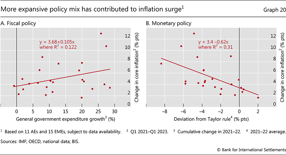
Monetary policy
While the central bank response to the inflation surge has been forceful and has clearly started to bear fruit, the job is not yet done. To be sure, tighter financial conditions have begun to weigh on expenditures, with economic activity slowing down most in interest rate-sensitive sectors. Labour markets have started to cool. And inflation expectations appear to have remained generally well behaved so far. That said, inflation is receding only slowly and the repeated forecast errors counsel caution in drawing firm inferences. Further, monetary policy is well known to operate with long and variable lags, making it difficult to pin down how large the impact has been so far. There is no room for complacency; perseverance is the name of the game.
Any assessment of the strength of policy transmission needs to consider the influence of factors that pull in different directions. On the one hand, higher debt levels, elevated asset prices and bursts of financial stress raise the sensitivity of the economy to tighter monetary conditions. Moreover, for the first time central banks are tightening not just through higher rates, but also by trimming their balance sheets. On the other hand, inflation-adjusted interest rates remain low or even negative and households and firms have been able to draw on the extraordinary support provided during the pandemic and on borrowing at longer maturities than in the past.
More fundamentally, the risk of shifting to a high-inflation regime greatly complicates the calibration of policy. Historical relationships no longer constitute reliable signposts.27 This makes the task of central banks much more difficult and can put their credibility on the line.
On balance, the biggest risk is to declare victory too soon. From a risk management perspective, policy rates may need to remain higher for longer to ensure that inflation continues to decline and stays low. Transitions to high-inflation regimes tend to be self-reinforcing and the trade-offs involved in restoring price stability worsen once inflation becomes entrenched. What’s more, history highlights the cost of stop-and-go actions, which can introduce unnecessary fluctuations in the economy. The costs of a high-inflation regime are simply too high to take any chances.
Support from other policies will be important for central banks to win the inflation fight, especially against the backdrop of elevated financial stability risks. Central banks can and should address financial stability risks without compromising the price stability objective. In the longer term, the two objectives do not pose a trade-off. But in the near term, the need to bring inflation back to target and the need to stabilise the financial system could pull in different directions. There will be a premium on differentiating central bank actions designed to achieve price stability from those aimed at financial stability – a task complicated by the extensive use of balance sheet policies to set the policy stance in several jurisdictions. If the stress is minor, central banks could address the near-term trade-off on their own, as the gilts market turmoil in the United Kingdom has shown.28 But if the stress is more acute, central banks will need the support of fiscal, prudential and supervisory policies to manage it effectively while retaining sufficient room for manoeuvre.29
Fiscal policy
The role of fiscal policy will be critical. To do its part, fiscal policy needs to consolidate. Consolidation would help tackle both the near-term and the longer-term challenges.
In the near term, consolidation would calm inflation by reducing pressure on productive capacity. And it would contain financial instability risks in several ways. It would reduce the need for monetary policy to tighten further. It would mitigate the risk that the sovereign itself becomes a source of financial instability, such as through the sovereign-bank nexus (Chapter II). And it would create more headroom should public resources be called upon for crisis management in concert with central banks.
In the longer term, consolidation would help rebuild the space necessary to put public sector debt on a firmly sustainable path. This is all the more important given the likelihood of greater demands on public spending, arising from ageing populations, the impact of geopolitical tensions on defence spending, and the green transition (Chapter II).
The recent policy record, however, highlights the risk of a drift in the fiscal stance. The design of the measures deployed to shield households and firms from the fallout of the war in Ukraine on energy and food prices leaves room for improvement. In general, it has not followed the “3T principle”, often for practical and political reasons. Support should be targeted to the most vulnerable groups so that the overall size is in line with the fiscal constraints and the needs of society. It should be tailored to ensure that it does not weaken incentives for needed medium-term adjustments. It should be temporary so as not to unduly add to demand after the shocks have passed.30 Moreover, any support boosts aggregate demand unless offset by higher taxes, regardless of how it is designed, thereby complicating the fight against inflation through that channel.
The recent improvement in fiscal positions reflects, to a considerable extent, only temporary factors. Even though fiscal expenditures exceeded original plans, primary deficits in G7 countries declined from 5.7% of GDP in 2021 to 3.4% in 2022. This largely reflected the inflation surge, which boosted both tax revenues and nominal GDP (Graph 21.A). These benign effects tend to be short-lived: they are one-off level adjustments. Further, it can prove politically difficult to withdraw support measures and the perception of a stronger fiscal position can tempt the authorities to spend rather than save the revenue windfalls.
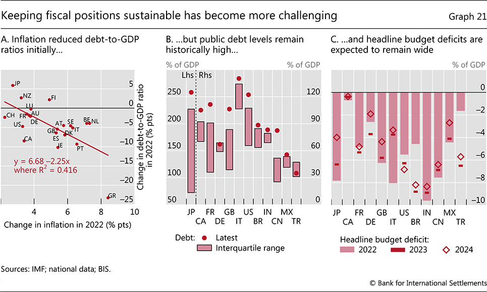
The ephemeral positive impact of inflation on debt ratios should not be exploited to avoid much-needed, credible consolidation plans. These plans should also aim to rationalise expenditures, improve the quality of spending and create space for supply side reforms (see Chapter II). Public-private partnerships should be part of the formula where possible. Absent consolidation, deficits remain too large to put public debt on a sustainable path. Debt levels in some major economies are at historical peaks or near them (Graph 21.B), and rising interest rates have increased the prospective debt service burden.
The challenge is daunting. To give a sense of the magnitudes involved, in 2019 a primary deficit of 2.1% of GDP would have been sufficient to stabilise debt, on average for G7 countries. In 2023, despite the one-off inflation-induced improvements in fiscal positions, higher interest rates mean that the corresponding figure has fallen to 1.6%. Among major EMEs, the debt-stabilising primary deficit has fallen from 1.1% of GDP in 2019 to 0.1%.31 While further shrinking of fiscal deficits is envisaged for most countries in 2023 and 2024 (Graph 21.C), these plans typically fall short of stabilising public debt even if they were meticulously followed. What is more, these figures assume that real long-term interest rates remain lower than real GDP growth rates, which cannot be relied upon. To reduce debt from its historically high levels, primary surpluses must clearly exceed the debt-stabilising ratios. Only this will restore fiscal space.
Prudential policy
Prudential policy, too, has an important role to play, in both the near and the longer term. By focusing on improving the resilience of the financial system, it can provide critical support to monetary and fiscal policies. Actions should address both banks and NBFIs.32 And they will need to be complemented by improvements in elements of the safety net as well as recovery and resolution schemes.
In the near term, the focus should be on actions that can quickly strengthen the loss-absorbing capacity of the financial system. This should be at both the macro- and the microprudential levels.
A premature easing of macroprudential measures should be avoided. Implemented before or during monetary policy tightening, such measures tend to reduce the likelihood of subsequent financial stress.33 It would be imprudent to ease them in anticipation of a slowdown in economic activity. In accordance with their design, they need to be kept in place and, where appropriate, tightened further and released only when clear risks of a disruptive credit crunch emerge.
At the microprudential level, a priority is tighter supervisory oversight. A culture of supervisory scrutiny should go beyond regulatory metrics and enforce timely remedial actions. Enforcement of stronger risk management practices, underpinned by sound governance, will be key. Given the build-up of indebtedness during the low-for-long era and the subsequent exceptional monetary policy tightening, losses could surpass forecasts based on historical data. This calls for conservatism in loan loss provisioning and in stress tests of exposures to interest rate, credit and liquidity risks.
Other adjustments will take more time.
In the banking sector, beyond the consistent and timely implementation of the post-GFC reforms, there is a need to learn from recent strains. In particular, lessons related to interest rate risk call for a reassessment of accounting rules and regulatory requirements. Historical cost accounting contributes to the accumulation of latent vulnerabilities when applied to assets that also serve liquidity management purposes (eg government securities). An overhaul of this practice would make reported capital more accurately reflect banks’ loss-absorbing resources. Furthermore, assumptions about the stickiness of various funding sources, most notably uninsured demand deposits, should be reassessed to improve banks’ liquidity requirements.
Beyond banking, there is an urgent need to strengthen the regulation of NBFIs from a systemic perspective. Deleveraging spirals and liquidity mismatches have exposed vulnerabilities that, if left unaddressed, could lead to broader systemic repercussions. A system-wide approach to strengthening NBFI resilience would need to build on a balanced mix of activity-based and entity-based regulatory requirements.34 Progress in this area has been disappointingly slow.
Turning to safety nets, an issue that has risen to prominence once again is the design of deposit insurance schemes. These schemes seek to safeguard the savings of retail depositors, who are unable to monitor financial intermediaries, and to facilitate the restructuring of failed banks. Together with central banks’ lender of last resort function, they also enhance the stability of banks’ funding, thereby supporting their ability to provide liquidity and manage maturity transformation.
Concerns about the rising structural instability of uninsured deposits has prompted calls for an expansion of the insurance coverage. Historically, it has proved very difficult to strike the appropriate balance. Arguably, however, experience indicates that, once confidence in an institution evaporates, deterring runs and preventing the institution from losing market access would require nothing short of insuring 100% of demandable and short-term claims, whether collateralised or not. This would encompass all forms of wholesale funding, including liquidity needs arising from margining practices. The upshot would be much weaker market discipline and, ultimately, a rise in solvency risks to unacceptable levels.
Hence, there is a premium on mechanisms to resolve institutions in an orderly way. Much progress has been made since the GFC in implementing the ambitious agenda concerning recovery and resolution frameworks. That said, further work is needed to equip authorities to manage bank failures more effectively. This entails closing the gap between available tools and the resolution requirements arising from banks’ scale, complexity or cross-border footprint. Key focus areas include facilitating the application of bail-in measures on all debt instruments with loss-absorbing features and establishing clear responsibilities and processes for the swift resolution of internationally active banks, especially G-SIBs. In addition, authorities should be in a position to address issues pre-emptively by steering banks towards sustainable business models.
Structural policies to enhance sustainable growth
Looking beyond the immediate challenges of inflation and financial stress, pre-pandemic sluggish growth could well set back in. Indeed, potential output growth estimates are at multidecade lows.35 There will then again be calls for monetary and fiscal policies to boost the economy’s prospects.
Experience offers valuable lessons, however, and indicates how misguided such calls can be. Policymakers should resist these calls. In the decades prior to the pandemic and the war in Ukraine, policymakers came to view the economy mainly through the lens of aggregate demand and assumed that aggregate supply adjusted smoothly in the background. The pandemic and the war were a rude awakening: supply side constraints do matter and macroeconomic policies stimulating aggregate demand to smooth the business cycle had largely run out of space.36 One lesson is that, to prevent unintended consequences, it is essential for monetary and fiscal policy to retain sufficient policy space and remain firmly within a region of stability (Chapter II).37 A second lesson is the need to reboot the supply side of the economy as the only possible source of robust, durable growth.
With a renewed focus on the supply side, policymakers need to identify the opportunities that longer-term trends can offer. The green transition, investments in state-of-the-art efficient facilities during the re-configuration of GVCs, digitalisation and the advancement of artificial intelligence could provide a much-needed push to productivity in many countries – provided that the right policies are in place.
A comprehensive approach to reap the potential benefits involves an array of structural policies. First and foremost, targeted investments in education should aim at continuous upskilling and re-skilling of the workforce. Adequate resources will need to be in place to ensure that workers can adapt and make effective use of the new technologies, so that the skills of a large part of the labour force do not become obsolete. In addition to education and training, policymakers should invest in healthcare, not only to mitigate any scarring effects from the pandemic and be prepared for other public health emergencies but also to maximise the productive potential of the workforce. Investments in human capital could be complemented by investments in physical capital. Infrastructure projects to improve connectivity and access to markets and services, when chosen carefully and implemented efficiently, could prop up productivity growth and enhance economies’ resilience. These investments may require not only better but also more public spending, further underscoring the need for fiscal consolidation through broadening of the tax base and entitlement reforms.
The other area of focus is maintaining competitive and open markets, both domestically and internationally. Economic structures are evolving rapidly, in response to the pandemic-induced shifts in preferences, geopolitical tensions, technological advances and climate change. Lowering barriers to entry would bring in new, innovative firms and help improve the outcomes of these transformations. Promoting free trade and resisting real and financial fragmentation would deliver better outcomes, given the important role trade has played in underpinning global productivity and growth.
Endnotes
1 For instance, in Brazil energy tax cuts are estimated to have lowered headline inflation by 2.5 percentage points in 2022 (Central Bank of Brazil (2022)). Estimates for France suggest that price caps and rebates have reduced headline inflation by about 3 percentage points between Q2 2021 and Q2 2022 (Bourgeois and Lafrogne-Joussier (2022)).
2 See Cavallino et al (2022).
3 This has given rise to the debate about “front-loading”; see Cavallino et al (2022) for an analysis.
4 These averages mask some variation, especially among EMEs: the tightening cycle of Latin American central banks pre-dated that of the Federal Reserve, while Asian economies typically embarked on tightening later, in part because the rise in inflation there was much more modest. Importantly, in China the official interest rate did not follow the global upward trend.
5 See Avalos et al (2022) for a discussion on the estimates of the growth impact under a natural gas shutdown scenario.
6 US banks seem to hedge little of their interest rate risk with derivatives, such as swaps (McPhail et al (2023)), in part due to reliance on hedges from their deposit franchise and accounting considerations.
7 In contrast to trading assets, changes to the market value of available-for-sale (AFS) and held-to-maturity (HTM) assets do not immediately have to be recognised in earnings. AFS and HTM assets, in turn, differ in how they affect banks’ reported equity, as this adjusts only in response to valuation changes on AFS holdings. In the United States, only the largest banks have to reflect such valuation changes in their regulatory capital. Following a change in legislation in 2018, banks with total assets of less than $250 billion, such as SVB before its failure, no longer have to reflect such losses.
8 See BIS (2022) and Borio et al (2023) for a detailed account of the transition mechanisms from a low- to high-inflation regime.
9 See Borio et al (2023).
10 See BIS (2022) for a historical perspective on how labour market institutions relate to low- vs high-inflation regimes.
11 Evidence exists of a negative and significant relationship between contract durations and inflation uncertainty. See Rich and Tracy (2004), Christofides and Peng (2006), Fregert and Jonung (2008).
12 See Cavallo and Kryvtsov (2023).
13 This interpretation comes with caveats. First, tight policy and weakened aggregate demand put a limit on profits. Second, a steady rise in profits and prices does not necessarily mean a steady rise in market power (captured by markups). Other factors, such as stronger demand or a temporary pause in new capital investment, could be behind the rising profits. Third, and related, margins 32 BIS Annual Economic Report 2023 and markups are notoriously difficult to measure accurately in real time and vary greatly among sectors. Last but not least, the link between market power and pass-through of costs to consumer prices is ambiguous. On the one hand, more power could allow firms to pass rising costs to consumers. On the other hand, higher markups could give firms headroom to absorb rising costs and compete on market share.
14 See Graph 9 in Borio et al (2023), which shows the sensitivity of inflation to past wage growth for different time periods. In addition, in Box 2 the authors use a cointegrating model for prices and wages to show that, in a high-inflation regime, changes in prices react in a significant way to changes in wages, and vice versa.
15 See Mojon et al (2023) for more details of the decomposition exercise and for a discussion of burden-sharing under projected disinflation paths in the euro area and the United States. In this simple accounting-based approach, profits are proxied by the ratio of GDP deflator to unit labour costs. Productivity growth is assumed to be in line with historical norms.
16 Of course, another margin of adjustment available to firms is the quantity rather than the price of labour. Typically, during disinflation episodes, unemployment increased about six months before peak headline inflation was reached and was almost 1.5 percentage points higher two years later. This time around, by contrast, unemployment actually fell as inflation rose and, to date, it has not risen much from the historically low levels it reached.
17 The sample covers Canada, Chile, Denmark, the euro area, India, Korea, New Zealand, Peru, Switzerland, Thailand and the United States.
18 The methodology and the underlying assumptions are explained in the technical annex. Notably, there is no explicit treatment of monetary policy. Its impact comes only indirectly: the exercise implicitly captures a successful monetary policy tightening by assuming that the unemployment gap returns to zero by the end of 2023 in all scenarios. Also, the results largely depend on the strength of the wage-price link estimated over a historical sample, and hence need to be taken with a pinch of salt: by considering the average strength of the relationship over a given sample, they may underestimate that, when inflation runs particularly high, the feedback effect may be even stronger.
19 See Igan et al (2022).
20 See Ampudia et al (2023).
21 Economies with relatively low debt levels tend to see house prices level off after the first rate hike, while those where household debt is in the upper third of the distribution typically see a pronounced and prolonged fall in house prices.
22 See FSB (2020).
23 ETFs could be less prone to such risks given their advantageous fund structure, see Shim and Todorov (2023).
24 The leveraged loans market also experienced strong growth, see Aramonte et al (2022).
25 See Aramonte and Avalos (2021).
26 For example, leveraged loan volumes reached multidecade highs in 2022, at more than $1.8 trillion in Europe and the United States. See Aramonte et al (2022).
27 For a discussion of how inflation indicators can become less useful during a regime switch, see De Fiore et al (2022). More generally, similar pitfalls plague the assessment of the current tightening. In a low-inflation regime, it may appear that monetary policy plays a minor role: as measured by standard models, the impact of monetary policy shocks – deviations from a policy rule – on inflation declines (eg Borio et al (2023)). This adds to the calibration challenge. But concluding that monetary policy as such does not matter would be a mistake: policy shocks do not capture the broader rule and the broader rule itself is what secures and maintains the low-inflation regime.
28 See Bailey (2023) for elaboration on a recent example.
29 See Chapter II on possible long-term adjustments to monetary policy frameworks to manage the trade-offs.
30 See OECD (2022) for an assessment of where different support measures stand on these dimensions. Governments often focus on price controls, which are in large part non-targeted, can blur price signals that would facilitate adjustment and tend to support rather than curb demand.
31 Simple averages of Brazil, China, India, Indonesia, Korea, Mexico and Poland.
32 See Carstens (2021).
33 See Boissay et al (2023).
34 See Borio et al (2022).
35 See IMF (2023) and OECD (2023).
36 See Carstens (2022).
37 See also Carstens (2023).
Technical annex
Graph 1: “Other AEs” is an average of AU, CA, CH, DK, GB, NO, NZ and SE, weighted by GDP and PPP exchange rates. “Latin America” is a simple average of BR, CL, CO and MX. “Other Asia” is a simple average of KR and SG. “Food and energy” includes alcoholic beverages.
Graph 3.A: Country groups calculated using GDP and PPP exchange rates. “AEs” is based on data for AU, CA, CH, DK, EA, GB, JP, NO, NZ, SE and US. “EMEs” is based on data for BR, CL, CN, CO, CR, CZ, HU, IL, KR, MX, PL, SA, TR and ZA. The coefficient of variation is calculated using data starting from 2012.
Graph 3.C: Calculation based on the principal component decomposition of the full sample. Nine AEs and eight EMEs.
Graph 4.A: For each country, tightening episodes are identified as months between the trough and peak in the policy rate around periods when the seven-month centred moving average of the policy rate is increasing. Episodes in which the policy rate increases by less than 1 percentage point or more than 20 percentage points, or episodes that last less than six months or more than 48 months, are excluded from the analysis. Based on data for 11 AEs and 16 EMEs from Jan 1970 to Feb 2023 (subject to availability); 154 tightening episodes.
Graph 4.B: Policy rate deflated by the weighted average of the current and next year Consensus forecasts for year-on-year inflation. Median based on monthly data for 11 AEs and 23 EMEs.
Graph 4.C Policy rate deflated by realised year-on-year inflation. Median based on monthly data for 11 AEs and 23 EMEs.
Graph 5.A: GDP-weighted average of EA, GB and US. Mortgage rates = for US, average of 15-year and 30-year fixed rate; for GB, average of two-year and five-year fixed rate with 60 and 90 LTV; for EA, new business mortgage rate. NFC loans rate = for US, bank prime loan rate; for GB, new business NFC fixed rate; for EA, new business NFC narrowly defined effective rate.
Graph 6.A: Country groups calculated as weighted averages using GDP and PPP exchange rates. “Other AEs” is based on data for AU, CA, CH, GB and SE. “EMEs excl CN” is based on data for AR, BR, CL, CO, CZ, HK, HU, ID, IL, IN, KR, MX, MY, PE, PH, PL, RO, RU, SA, SG, TH, TR, VN and ZA.
Graph 7.A: “EMEs” is based on data for AE, AR, BR, CL, CO, CZ, DZ, HU, ID, IL, KR, MA, MY, MX, PE, PH, PL, RO, RU, SA, SG, ZA, TH and TR. Calculated as weighted averages using GDP and PPP exchange rates.
Graph 7.C: For economic activity, Yicai Research Institute’s high-frequency economic activity indicator; for box office revenues, one-month rolling average of the Maoyan Entertainment’s box office revenues; for port congestion, the average of Kiel Institute’s traffic indices for Hong Kong SAR and Guangdong, and for Shanghai and Zhejiang; for road congestion, the one-month rolling average of the average China Ministry of Transport’s road congestion index across 101 Chinese regions; for subway traffic, the one-month rolling average of the sum of number of passengers in 10 important Chinese regions; for international flights, the one-month rolling average of the number of operated international flights.
Graph 9.A: S&P 500 index for the United States; Shanghai Shenzhen CSI 300 Equity Index for China. AEs (excl US): weighted average of S&P/ASX 200, S&P/TSX Composite Index, Swiss Market Index, OMX Copenhagen Index, EURO STOXX 600 Index, FTSE 100 Index, Nikkei 225, OBX Stock Index, S&P/NZX 50 Index and OMX Stockholm Benchmark for AEs. EMEs (excl CN): weighted average of Brazil Ibovespa Index, S&P/CLZ IPSA, MSCI Colcap Index, Prague Stock Exchange Index, Hang Seng Index, Budapest Stock Exchange Index, S&P BSE Sensez Index, Jakarta Composite Index, Kospi Index, S&P/BMV IPC Index, FTSE Bursa Malaysia KLCI, S&P/BVL PeruGeneral TRPEN, PSEi Philippine SE Index, WSE WIG Index, Straits Times Index, Stock Exchange of Thailand Index and FTSE/JSE Africa ALL SHR Index for EMEs.
Graph 10.A: Long-duration loans, mortgages and debt securities as a percentage share of total loans, mortgages and debt securities; based on a sample of more than 230 large and mid-size US banks.
Graph 10.B: Estimated impact of a +200 basis point parallel shift in the yield curve on banks’ Tier 1 capital; “Other” comprises G-SIBs from Canada, China and Japan; based on available G-SIB disclosures at end-2022 and end-2021 data for Silicon Valley Bank (SVB).
Graph 10.C: Regional aggregates based on a balanced sample of 341 major banks from 42 countries; four-quarter rolling averages.
Graph 11.A: Outstanding loans through the Federal Reserve’s Bank Term Funding Program and discount window (primary credit) up to latest available.
Graph 11.B: Asset-weighted average based on a sample of 233 US banks.
Graph 12: Each disinflation episode is captured when the 13-month moving average is at its peak, under the conditions that (i) there are no other peaks in the preceding and the following 12 months; (ii) the peak is between 3% to 25%; and (iii) the peak is at least 3 percentage points higher than the lowest troughs in the preceding and the following 12 months. Month = 0 is when the actual headline inflation value is at the highest during that particular episode. Panel of 30 AEs and 28 EMEs, subject to data availability. In Graph 12.D, real interest rate is computed as an ex post rate using the policy rate and the headline inflation.
Graph 13.B: High-inflation regime samples: CA, Q4 1971–Q4 1990; JP, Q4 1970–Q4 1979; KR, Q4 1985–Q4 1997; MX, Q1 1983–Q4 2002; US, Jan 1965–Dec 1985. Low-inflation regime samples: CA, Q1 1991–Q4 2019; JP, Q1 1980–Q4 2019; KR, Q1 1998–Q4 2019; MX, Q1 2003–Q4 2019; US, Jan 1986–Dec 2019.
Graph 14.B–C: See technical annex for Graph 12 for the definition of disinflation episodes. Real wages are computed by deflating nominal wages by headline CPI. Profits are proxied by the ratio of GDP deflator to unit labour costs.
Graph 15.A: Projections are based on country-specific macroeconomic models, the results of which are then aggregated using GDP weights. The models estimate a long-run relationship between the (log-)level of prices (core CPI), wages (average hourly compensation for total economy) and labour productivity, as well as short-run adjustment equations in which deviations from the long-run relationship contribute to the dynamics; the models and the estimates are described in detail in Borio et al (2023), Box B. Conditional projections of inflation are constructed by letting labour productivity grow at the average rate observed over the last 10 years, and assuming a wage growth rate as specified under each of the two scenarios. For the projections in 2023, average residuals of inflation in 2022 are also included, decaying by a factor of 0.25 every quarter. Note that, since core CPI is used as the metric for prices, import prices drive a wedge relative to an exercise where the GDP deflator is used.
Graph 18: Projections are based on country-specific macroeconomic models. The models consist of a VAR linking the behaviour of private sector debt-to-income ratios, real house prices, real equity prices, real income, effective private sector interest rates and real GDP. The coefficients in some VAR equations (eg equity prices) are restricted to reflect realistic information lags. VARs are estimated over the sample Q1 1985–Q4 2019. Policy interest rates are included as an exogenous variable in the model. In each scenario, all variables other than the policy rate evolve according to their estimated relationships in the model.
Graph 19.A–B: Credit losses calculated based on the private sector debt-to-income and credit growth projections shown in Graph 17 using the approach described in Juselius and Tarashev (2022).
Graph 19.C: Total capital ratio is the total capital adequacy ratio under the Basel III framework. It measures Tier 1 plus Tier 2 capital, which includes subordinated debt, hybrid capital, loan loss reserves and the valuation reserves as a percentage of risk-weighted assets and off-balance sheet risks.
References
Ampudia, M, F De Fiore, E Kharroubi and C Manea (2023): “Private debt, monetary policy tightening and aggregate demand“, BIS Bulletin, no 70, February.
Aramonte, S and F Avalos (2021): “The rise of private markets“, BIS Quarterly Review, December, pp 69–82.
Aramonte, S, K Todorov and K Detering (2022): “Are CLO investors underestimating tail risk in European markets?”, BIS Quarterly Review, September, pp 13–14.
Avalos, F, A Cap, D Igan, E Kharroubi and G Nodari (2022): “Energy markets: shock, economic fallout and policy response“, BIS Bulletin, no 64, December.
Bailey, A (2023): “Monetary and financial stability: lessons from recent times”, speech at the Institute of International Finance, 12 April.
Bank for International Settlements (BIS) (2022): “Inflation: a look under the hood“, Annual Economic Report 2022, June, Chapter II.
Baron, M, E Verner and W Xiong (2021): “Banking crises without panics”, Quarterly Journal of Economics, vol 136, no 1, pp 51–113.
Boissay, F, C Borio, C Leonte and I Shim (2023): “Prudential policy and financial dominance: exploring the link“, BIS Quarterly Review, March, pp 15–31.
Borio, C, S Claessens and N Tarashev (2022): “Entity-based vs activity-based regulation: a framework and applications to traditional financial firms and big techs“, FSI Occasional Papers, no 19.
Borio, C, M Lombardi, J Yetman and E Zakrajšek (2023): “The two-regime view of inflation“, BIS Papers, no 133, March.
Bourgeois, A and R Lafrogne-Joussier (2022): “La flambée des prix de l’énergie: un effet sur l’inflation réduit de moitié par le «bouclier tarifaire»”, Insee Analyses, no 75, September.
Caparusso, J, Y Chen, P Dattels, R Goel and P Hiebert (2019): “Post-crisis changes in global bank business models: a new taxonomy”, IMF Working Papers, WP/19/295.
Caparusso J, U Lewrick and N Tarashev (2023): “The long-run profitability and resilience of globally systemic banks”, BIS Bulletin, forthcoming.
Carstens, A (2021): “Non-bank financial sector: systemic regulation needed“, Foreword, BIS Quarterly Review, December, pp 1–6.
— (2022): “A story of tailwinds and headwinds: aggregate supply and macroeconomic stabilisation“, speech at the Federal Reserve Bank of Kansas City Jackson Hole symposium, 26 August.
— (2023): “Monetary and fiscal policies as anchors of trust and stability“, speech at Columbia University, New York, 17 April.
Cavallino, P, G Cornelli, P Hördahl and E Zakrajšek (2022): “‘Front-loading’ monetary tightening: pros and cons“, BIS Bulletin, no 63, December.
Cavallo, A and O Kryvtsov (2023): “What can stockouts tell us about inflation? Evidence from online micro data”, Journal of International Economics, https://doi.org/10.1016/j.jinteco.2023.103769.
Central Bank of Brazil (2022): Inflation Report – September 2022.
Christofides, L and A Peng (2006): “Contract duration and indexation in a period of real and nominal uncertainty”, Labour Economics, vol 13, issue 1, pp 61–86.
De Fiore, F, M Lombardi and D Rees (2022): “Inflation indicators amid high uncertainty“, BIS Bulletin, no 60, September.
Financial Stability Board (FSB) (2020): “Global Monitoring Report on Non-Bank Financial Intermediation”, Financial Stability Board Report, 16 December.
Fregert, K and L Jonung (2008): “Inflation targeting is a success, so far: 100 years of evidence from Swedish wage contracts”, Economics Discussion Paper, no 2008-24.
Goel, T, U Lewrick and A Mathur (2021): “Does regulation only bite the less profitable? Evidence from the too-big-to-fail reforms“, BIS Working Papers, no 922.
Hofmann, B, T Park and A Tejada (2023): “Commodity prices, the dollar and stagflation risk“, BIS Quarterly Review, March, pp 33–45.
Igan, D, E Kohlscheen and P Rungcharoenkitkul (2022): “Housing market risks in the wake of the pandemic“, BIS Bulletin, no 50, March.
International Monetary Fund (IMF) (2023): World Economic Outlook, April.
Juselius, M and N Tarashev (2022): “When uncertainty decouples expected and unexpected losses“, BIS Working Papers, no 995, January.
Laeven, L and F Valencia (2020): “Systemic banking crises database II”, IMF Economic Review, vol 68, January, pp 307–61.
McCauley, R and C Shu (2019): “Recent renminbi policy and currency co-movements”, Journal of International Money and Finance, vol 95(C), July, pp 444–56.
McPhail, L, P Schnabl and B Tuckman (2023): “Do banks hedge using interest rate swaps?” NBER Working Papers, no 31166.
Mink, M, J Jacobs and J De Haan (2007): “Measuring synchronicity and co-movement of business cycles with an application to the euro area”, Cesifo Working Papers, no 2112, October.
Mojon B, G Nodari and S Siviero (2023): “Disinflation milestones“, BIS Bulletin, no 75, May.
Organisation for Economic Co-operation and Development (OECD) (2022): “Special feature: policy responses to rising energy prices”, Tax Policy Reforms 2022: OECD and Selected Partner Economies.
— (2023): Economic Policy Committee report, May.
Rich, R and J Tracy (2004): “Uncertainty and labor contract durations”, The Review of Economics and Statistics, vol 86, no 1, pp 270–87.
Shim, J and K Todorov (2023): “ETFs, illiquid assets, and fire sales”, BIS Working Papers, forthcoming.
II. Monetary and fiscal policy: safeguarding stability and trust

BIS Annual Economic Report |
![]() Watch the video (00:02:20)
Watch the video (00:02:20)
with Claudio Borio, Head of the Monetary and Economic Department
Listen to the podcast (00:26:06)
with Claudio Borio
Key takeaways
- As core economic functions of the state, monetary and fiscal policy are inextricably intertwined.
- To be conducive to a stable financial and macroeconomic environment and keep tensions between them manageable, the policies need to operate within a “region of stability”. The ultimate risk of drifting outside the region is a loss of the trust that society must have in the state and in its decision-making.
- In recent decades, monetary and fiscal policy gradually moved towards the boundaries of the stability region, as they were often relied upon as de facto engines of growth. This has set the stage for the current tensions between them, as well as for the macroeconomic and financial risks ahead.
- Policy adjustments and institutional safeguards are needed to ensure that the two policies remain firmly within the region of stability. These hinge on a keener recognition of the limitations of macroeconomic stabilisation policies.
Introduction
For the first time in recent decades, we are seeing high inflation and financial stress emerging in tandem. While each has its own specific causes (Chapter I), they are, to a significant extent, a symptom of the cumulative effect of accommodative monetary and fiscal policy over past decades, culminating in the extraordinary support measures launched in response to the pandemic. In many countries, policy rates, nominal and real, were historically low for a prolonged period and central bank balance sheets surged to levels never seen in peacetime (Graph 1.A). At the same time, persistent and large fiscal deficits led to a progressive increase in public debt to unprecedented levels (Graph 1.B). These policy trajectories gave an important and enduring push to inflation and fostered the build-up of fragilities in the financial system.1
The current tensions can be seen as a symptom that the two policies were testing the boundaries of what might be called the “region of stability”. The region maps constellations of monetary and fiscal policy that foster macroeconomic and financial stability, and keep the inevitable tensions between the policies manageable. The region’s boundaries are elusive and it is often only fully apparent ex post that they have been tested, since economic systems can appear stable until, suddenly, they are not. The ultimate risk of drifting outside the region is a loss of the trust that society must have in the state and in its decision-making.
The recent challenge to the boundaries is the latest in a long journey that stretches back to at least the 1970s. At each point in time, the policy choices seemed reasonable, even compelling. But cumulatively, they pushed the policies towards the boundaries. The root cause of the drift has been a tendency for policymakers to succumb to a kind of “growth illusion”, ie an overly optimistic view about the ability of macroeconomic stabilisation policies to sustain economic growth.2
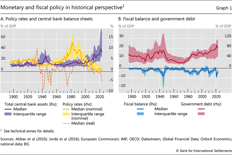
Policy adjustments and institutional safeguards are needed to ensure that monetary and fiscal policy remain firmly within the region of stability. The policies should aim to foster a stable financial and macroeconomic environment in which sustainable growth, which is ultimately driven by supply factors, can take hold. And, to do so, they need to retain sufficient safety margins to deal with unexpected untoward events, as well as inevitable recessions. Ultimately, though, the adjustments call for a shift in mindset, that is, a keener recognition of the limitations of stabilisation policies, which cannot act as engines of growth. Having the region of stability as a conscious and explicit policy consideration would help to guide action.
This chapter lays out the enduring challenge for monetary and fiscal policy to stay within the region of stability and how it might be addressed. The chapter first outlines the role of monetary and fiscal policy as core economic functions of the state and introduces the concept of the region of stability. It then describes the journey of monetary and fiscal policy over the past decades to the boundaries of the region, ushering in high inflation and financial fragility. It next discusses the potential risks ahead for macroeconomic and financial stability. The chapter ends by exploring policy implications.
Policy interactions and the region of stability
As two core economic functions of the state, monetary and fiscal policy play a key role in ensuring economic stability and trust in policymaking. Both policies entail privileged powers to access and reallocate economic resources in society. Fiscal policy hinges on the power to raise taxes and the prerogative to issue debt backed by future tax revenues. Monetary policy wields the power to issue “money”, an irredeemable liability of the state used as a means of payment. These powers are mutually reinforcing. The requirement to pay taxes with money sustains money demand, encouraging its use as a payment tool. In turn, a stable monetary system strengthens the tax base. Furthermore, money issuance supports fiscal revenues through seigniorage and can help prevent technical government default as public debt is redeemable against money.
The privileged powers of fiscal and monetary policy ultimately depend on an implicit social contract underpinned by trust in the state. People consent to paying taxes because they trust the government to use the proceeds for the public good. Similarly, people accept the use of money as a means of payment because they trust the central bank to preserve its value.
Box A
The consolidated central bank-government budget constraint
The balance sheets of the central bank and the government are joined at the hip. This, in turn, tightens the link between monetary and fiscal policy and can blur the distinction between them. The balance sheets are intertwined because the central bank is “owned” by the government or is part of it, sending to it remittances based on the institution’s financial results. In addition, it is quite common for the two organs of the state to hold claims on each other and issue others that are very close substitutes in private sector portfolios. Examining the link between the two balance sheets sheds further light on the interaction between the two policies.
Consider first the central bank’s balance sheet. Its assets typically consist of government securities, claims on the private sector (eg lending to banks) and (often but not always) foreign currency reserves. Its liabilities take the form of own debt (eg own paper or reverse repos) and “monetary liabilities”, ie cash in the hands of the public and bank reserves – the “monetary base”. Very often, they may also include government deposits. The residual between the value of the assets and liabilities is the central bank’s capital. The balance sheet of the fiscal authority includes the central bank’s capital as an asset, as well as any other assets held, and liabilities issued, by the fiscal authority.
Consolidating the two balance sheets highlights two important points.
First, large-scale central bank purchases of long-term government debt amount to a large debt management operation, the nature of which depends on how the central bank finances them. Since cash is entirely demand-determined, the central bank can either issue its own short-term debt – almost indistinguishable from that of the government – or increase the amount of bank reserves. However, if the central bank wishes to retain control over the interest rate, those reserves must be interest-bearing: the interest rate would fall to zero for as long as those reserves are not reabsorbed. The reserves are, in fact, indexed to the overnight rate.
Second, central bank profits and losses feed through to the government’s financial position. This can strengthen or weaken it in ways that would not be apparent if one considered only the government’s financial accounts. For instance, the government may lengthen the maturity of its liabilities. But if the central bank purchased an equivalent amount, the corresponding government debt would be, in effect, overnight or short-term. This would raise, not lower, the sensitivity of the fiscal position to higher interest rates. The higher sensitivity would show up as greater interest costs to the central bank and, through lower remittances to the fiscal authority, lower government revenues.
One example helps to illustrate these two points (Graph A1). Assume that the government issues more long-term (fixed rate) bonds to finance the acquisition of long-term assets, such as public infrastructure (Graph A1.A). Next assume that the central bank buys this debt and finances it by issuing remunerated overnight bank reserves (Graph A1.B). Looking at the balance sheet of the government alone, it would appear that the government has lengthened the maturity of its debt and reduced the sensitivity of its funding costs to higher interest rates. In reality, looking at the consolidated balance sheet, it is clear that the sensitivity is now higher, as higher interest rates immediately reduce central bank remittances (Graph A1.C). In case of large capital losses by the central bank, remittances may even become negative.
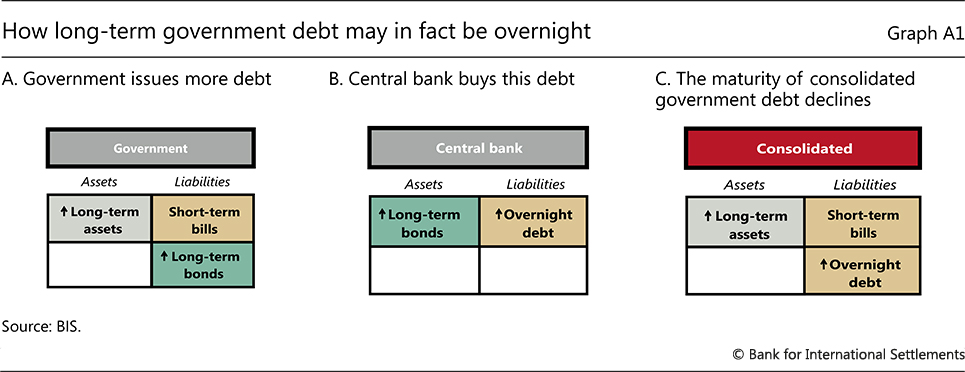
Considering the evolution of the consolidated balance sheet in stylised form sheds further light on how fiscal and monetary policies interact. The budget constraint can be written as follows:
 where Dl,t is the consolidated domestic currency debt (including any central bank debt and interest-bearing bank reserves); Df,tEt is the consolidated foreign currency net debt (ie debt minus FX reserves) expressed in domestic currency (Et is the exchange rate); rl,t and rf,t are the corresponding interest rates; PBt is the primary balance (taxes minus spending excluding interest payments); and ΔMt is the change in (non-interest-bearing) monetary liabilities (reserves and cash). All the variables are expressed in nominal terms. Dividing by nominal GDP and combining the domestic and foreign currency components of net debt, highlights the factors determining the evolution of the net debt-to-GDP ratio:
 where pbt and st = ΔMtYt are the primary balance and so-called seigniorage as a share of GDP, respectively, and gt is the growth rate of nominal GDP. Note that the effective interest rate rt is a weighted average of the interest rate paid on domestic and foreign currency debt (with at indicating the share of domestic currency debt in total net debt) and includes valuation effects through the depreciation et of the exchange rate:
 The consolidated debt-to-GDP ratio shifts the region of stability. All else equal, as the ratio increases, the region narrows, since a smaller set of interest rates and fiscal balances is consistent with macroeconomic and financial stability. The key variables in (2) are the primary balance and the difference between the yield on the debt and the nominal growth rate of the economy – the so-called growth-adjusted interest rate. Whenever positive, this difference tends to increase the debt-to-GDP ratio over time, at a rate that increases with the debt level. Even primary surpluses may not be large enough to offset this effect (see Box C for a detailed discussion). Seigniorage can be largely ignored when inflation is low: it is small and, in contrast to the nominal interest rate, demand-determined and hence not under the control of the central bank. Non-monetary liabilities evolve broadly in line with GDP. This adds nuance to the ambiguous notion of “monetary financing”.
Thus, the consolidated budget constraint highlights that monetary and fiscal policy are inextricably linked. Higher interest rates as, say, may be needed to address inflation, weaken the fiscal position and, if this is precarious enough, can generate strains. By the same token, a fragile fiscal position reduces the monetary policy room for manoeuvre, as it makes the control of inflation more costly. Indeed, in the case of acute concerns about the sovereign’s creditworthiness, monetary policy could even lose control of inflation altogether. The concerns could trigger a run on government debt, capital flight and a sharp depreciation of the currency, which would generate inflation. A sharp tightening of monetary policy would simply intensify concerns about a possible default, especially if part of the debt was denominated in foreign currency. Even if default was avoided, this would be at the cost of higher, most likely runaway, inflation. Ultimately, maintaining low and stable inflation requires fiscal backing.
The central bank could also increase a non-interest-bearing reserve requirement, which is a form of tax on the banking system. Here M does not correspond to the monetary base or M0, as the latter also includes interest-bearing reserves. Specifically, the demand for cash is largely a demand for transactions balances: it can be thought to depend on nominal income and, with limited sensitivity, on the nominal interest rate. That for non-interest-bearing reserves is either minimal or depends on the factors driving any reserve requirements, typically the deposit base to which they are related. Deposits, too, can be thought of as a function of the same variables as cash. In the majority of episodes of high inflation and hyperinflation, the root cause was often a fiscal imbalance and/or an unrealistic target for the exchange rate coupled with an accommodative response of the central bank. See eg Fischer et al (2002). The crucial role of fiscal policy in determining inflationary outcomes is at the heart of the fiscal theory of the price level (FTPL). Any increase in government debt that is not backed by the credible expectation of higher future fiscal surpluses creates inflationary pressures, with default being ruled out as too costly. The underlying mechanism that pushes the price level up is a wealth effect. See eg Cochrane (2023) for a description of the FTPL and additional examples.
The need to retain society’s trust sets limits on the privileged powers of the two policies. Monetary and fiscal policies can become a major force for prosperity if used effectively to provide public goods and to ensure a stable financial and macroeconomic environment, underpinned by a sound payment system. If instead their powers are wielded unwisely, the policies can seriously damage the economy and, ultimately, trust in the state.
The main channels through which monetary and fiscal policies influence economic activity differ considerably. Fiscal policy does so primarily through the direct impact of spending on goods and services, and the production of some of those services, as well as through transfers to households and firms. Monetary policy works primarily through the central bank’s operations in financial markets – notably the policy interest rate – which have a pervasive effect on yields, borrowing costs, asset prices and the exchange rate.
That said, overlaps are also substantial. Fiscal policy influences financial conditions through debt issuance. Not only does public debt underpin the functioning of the financial system and the pricing of assets, it can have a far-reaching effect on the yield curve, other asset prices and the exchange rate, as well as on the soundness of the financial system when fiscal soundness is put in doubt. Monetary policy, in turn, influences the state of public finances. It does so directly, by setting interest rates (borrowing costs) and through its effect on the exchange rate (when debt is denominated in foreign currency); and it does so indirectly, through its impact on economic activity and inflation more generally, which can materially alter government expenditures and taxes.
The two policies are further entwined through interlocking balance sheets (Box A). Since the central bank is part of the state, its financial results feed into the financial condition of the government through remittances. The large-scale purchases of government debt, as well as the accumulation of foreign exchange reserves, have made government finances more sensitive to central bank decisions.
The region of stability
The pervasive impact that monetary and fiscal policy have on economic activity, and the overlapping nature of their transmission channels, means that the two policies are joined at the hip. They may work in a coherent fashion to foster a stable financial and macroeconomic environment; but they can, equally, undermine that stability and generate tensions between them that are very difficult to manage.
The concept of the “region of stability” helps identify the appropriate zone of operation of the two policies (Box B).3 This region captures the set of monetary and fiscal policies that are consistent with macroeconomic and financial stability. The boundaries of the region vary across countries and are difficult to pin down with precision ex ante. They cannot be summed up in simple metrics, akin to a constraint on the level of the fiscal deficit or on the policy rate.
Furthermore, the size, shape and locus of the region shift over time. Some changes occur gradually, such as those due to structural developments in the labour market and the structure of production. But the region can also shrink and shift position rapidly, for example due to a sudden loss of confidence in policy or in the economy at large – a risk that has become more acute over time due to the rapid growth and increased fragility of the financial system. This underscores the need for fiscal and monetary policy to operate well within the region and to leave sufficient safety margins at its boundaries.
Box B
The region of stability and its determinants
The region of stability identifies the set of fiscal and monetary policy combinations which are consistent with macroeconomic and financial stability. When fiscal and monetary policies operate within this region, tensions between the two policies may arise frequently but remain manageable. However, when fiscal and monetary policies approach the boundaries of the region, they encroach on each other and endanger macro-financial stability.
A key challenge for policymakers is that the region of stability evolves over time in size, shape and position (Graph B1.A). In certain periods, the region can be quite extensive, encompassing a broad set of monetary and fiscal settings. But the region can then rapidly shrink. Monetary and fiscal policy combinations that appear consistent with macro-financial stability at a given point in time, may, all of a sudden, no longer be.
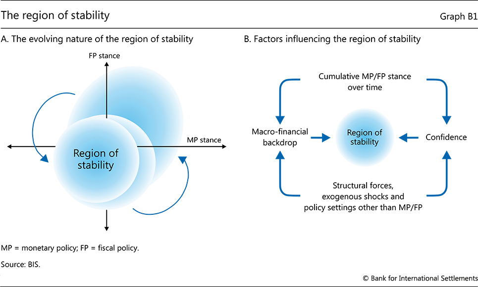
Several factors influence the region of stability by changing the macro-financial backdrop and the degree of public confidence in the economic outlook and in the soundness of the policy framework (Graph B1.B). Some of these factors are relatively slow-moving. For example, structural forces – including technological and financial innovation – can gradually alter the foundations of production and finance, in turn shaping the set of monetary and fiscal policies that are consistent with macro-financial stability. Demographic factors can also slowly but profoundly change labour markets. And international trade and financial integration – or forces that work against it – can heavily influence the global economic landscape and thus the room for fiscal and monetary policy manoeuvre.
But other factors can evolve much faster, abruptly shifting the locus and size of the region of stability. One possibility is sudden exogenous shocks. For example, the commodity price surge triggered by the Russian invasion of Ukraine provides a vivid illustration of such a risk. Furthermore, confidence effects greatly heighten the potential for sudden movements in the region. Market sentiment and public trust in the ability of macroeconomic policies to preserve stability can shift rapidly and, in turn, dramatically narrow the fiscal and monetary space. A sharp depreciation of the exchange rate is often the first sign of a loss of confidence as well as a key channel that constrains the policy headroom.
The rapid growth of the financial system in recent decades has made sudden shifts in the region of stability more likely. By becoming more sophisticated and fast-paced, the system has also become increasingly fragile. Leverage and liquidity mismatches have ballooned, in plain sight as well as out of sight. In such a system, confidence can suddenly evaporate, bringing about runs on financial institutions and market breakdowns. This fragility can abruptly shrink the region of stability by limiting the set of fiscal and monetary policy combinations that are consistent with investor confidence.
Besides being affected by structural forces and exogenous shocks, policies other than monetary and fiscal ones exert a heavy influence on the region. For example, microprudential and macroprudential regulation play a critical role in limiting financial excesses and building precautionary buffers, thus preserving greater space for fiscal and monetary policy. A targeted and well calibrated use of foreign exchange rate interventions, in some situations possibly complemented by capital flow management measures, may also enhance macroeconomic resilience, and provide fiscal and monetary policy with greater flexibility. And structural reforms can considerably expand the region by boosting potential growth, thereby reducing public pressures for monetary and fiscal policies to support economic activity.
Yet an even more important – although much less appreciated – aspect is that the cumulative impact of fiscal and monetary policies themselves can profoundly alter the region of stability. Policy settings that may appear stabilising in the near term can, over time, inadvertently shrink the region. For example, monetary and fiscal settings with expansionary effects in the short term may come at the cost of higher instability down the road by encouraging leverage and risk-taking. Prolonged policy accommodation may also create misperceptions about economic fundamentals. An extended period of easy monetary conditions when inflation is held down by favourable tailwinds may provide the false impression of a permanent and independent decline in real rates that can lure policymakers towards the region’s boundaries.
The concept of the region of stability thus underscores the critical intertemporal trade-offs associated with fiscal and monetary policy. In setting policy, policymakers should not only remain firmly within the region of stability but they should also ensure that the cumulative impact of fiscal and monetary settings does not shrink the region over time. Failure to do so can have severe consequences, by dramatically narrowing the space for policy manoeuvre, heightening tensions between monetary and fiscal policies, and ultimately undermining macro-financial stability and trust in the key functions of the state.
See Borio and Disyatat (2021) for an early discussion on how the region of stability constrains and is in turn affected by fiscal and monetary policy. Structural factors – including rising inequality, an ageing population and decreases in technological progress – have been proposed as possible drivers of the decline in real interest rates. See eg the discussion in Blanchard (2022). Yet the empirical evidence is weak. See Borio et al (2017). These concepts are at the centre of the literature on currency crises, eg Krugman (1979), Obstfeld (1996) and Aghion et al (2004). See eg Farhi and Werning (2016), Cerutti et al (2017), Korinek and Simsek (2016) and Bergant et al (2023). See eg Cavallino and Sandri (2023) and Bianchi and Lorenzoni (2022). High public and private leverage may, for example, constrain monetary policy and undermine macroeconomic stability via fiscal and financial dominance concerns, as articulated for example in Sargent and Wallace (1981) and Brunnermeier (2015). Evidence regarding the link between credit growth and subsequent financial crises is presented in Borio and Lowe (2002) and Schularick and Taylor (2012). For models in which monetary easing may drive a prolonged reduction in real interest rates, see Rungcharoenkitkul et al (2019), Mian et al (2021) and Kashyap and Stein (2023). Evidence about the effects of monetary policy on long-term real rates is provided in Borio et al (2019), which also includes a review of the literature.
The cumulative effect of past fiscal and monetary policy decisions crucially shapes the region’s boundaries. For example, prolonged periods of monetary and fiscal accommodation may contribute to the build-up of a broad range of vulnerabilities – including greater leverage and risk-taking – that can eventually constrain the policies’ room for manoeuvre. Hence the typically intertemporal nature of the trade-offs involved. A policy conduct that may appear stabilising in the near term can, over time, inadvertently shrink the region and take policies towards the boundary. The economic system may appear stable for a long time until, suddenly, it is not.
The boundaries are also approached through the interaction of the two policies. For a given interest rate path, a fiscal policy stance that is cumulatively too loose will risk higher inflation and a sovereign crisis, as debt builds up. For a given fiscal policy path, a monetary policy stance that is cumulatively too easy can generate higher inflation and financial stability risks. Along the corresponding paths, the two policies can reinforce each other’s trajectories. Easy monetary policy can induce the government to build up more debt; expansionary fiscal policy can make it harder for monetary policy to be as tight as necessary.
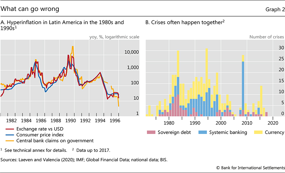
Testing the region’s boundaries can trigger vicious cycles. In that case, both policies end up narrowing their respective rooms for manoeuvre, shocks become increasingly damaging and policies increasingly destabilising. The instability, in turn, threatens or reflects loss of trust in the policies themselves. A common feature is loss of trust in money – as a store of value, means of payment or unit of account – and in the sustainability of public debt.
Instability in the wake of overstepping the boundaries of the region of stability can take different forms. Common manifestations include high inflation, economic slumps, sovereign default and financial stress. A sharp depreciation of the exchange rate is a typical symptom and transmission channel. The most acute manifestation of drifting far outside the boundaries is hyperinflations, such as those experienced in some Latin American emerging market economies (EMEs) in the 1980s and 1990s. These show how fiscal pressures and their monetary policy accommodation can destroy the value of money (Graph 2.A).
Another manifestation is the coincidence of sovereign debt, systemic banking and currency crises (Graph 2.B). Acute financial crises often feature the so-called doom loop between the sovereign’s balance sheet and the financial sector. In such episodes, fiscal and financial instability reinforce each other, as banks suffer losses on government bond holdings while governments need to shore up the failing banking system. In turn, these fiscal and financial crises undermine trust in the currency, and currency depreciation further exacerbates instability.
Testing the boundaries: the long journey so far
The journey: from the 1960s to today
Prior to the pandemic, monetary and fiscal policy were already approaching the boundaries of the region of stability. Interest rates had been historically low for a prolonged period and central bank balance sheets had risen to wartime-like levels following more than a decade of monetary stimulus in the wake of the Great Financial Crisis (GFC). At the same time, public debt had reached historical highs following persistent fiscal deficits. This constellation meant a substantial loss in room for policy manoeuvre and left economies vulnerable to shocks as well as to the inevitable next recession. Then, when the pandemic – a bolt from the blue – struck, the policies tested those boundaries further, ushering in high inflation and financial fragility.
How did monetary and fiscal policies come to approach the boundaries pre-pandemic? It was the result of a long journey. The journey was not linear. The symptoms of an overly expansionary policy stance evolved with the economic landscape that those policies were helping to shape, together with more fundamental structural forces. A consistent underlying factor was the overestimation of how far macroeconomic policies could steer the economy and, by pushing hard enough, ignite the engine of growth – a kind of “growth illusion”. This induced a progressive loss of policy space over time.
It is useful to divide the journey going back to the 1960s into two phases, with the mid-1980s as a rough watershed. Graph 3 illustrates the break, with reference to advanced economies (AEs) – see below for a discussion of similarities and differences with EMEs.
Until the mid-1980s, the key symptom indicating that the policies were testing the speed limits of the economy, and hence the boundaries of the region of stability, was rising inflation. Recessions were typically induced by a tightening of monetary policy to quell inflation. With the financial system hemmed in by regulation, signs of large build-ups and contractions in credit were missing. During this phase, the drift to the boundaries reflected, in part, the belief that policymakers could fine-tune the economy by a carefully calibrated mix of monetary and fiscal policy. Hence the concept of a stable long-run trade-off between unemployment and inflation. The result was the Great Inflation of the 1970s.
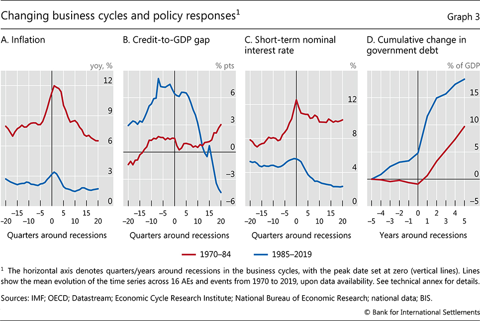
In response to the inflation crisis, policymakers took steps to bring monetary and fiscal policies back within the region of stability. Central banks sought to end inflation by aggressively hiking policy rates. Following the disinflation in the first half of the 1980s, monetary regimes prioritising price stability gradually became the norm. Interest rates declined substantially from their previous peak. However, the rise in interest rates on the back of monetary tightening in the early 1980s had exposed fiscal fragilities in many countries. In combination with persistent fiscal deficits, this led to a surge in public debt. Thus, many governments were forced to embark on fiscal consolidation. For more than a decade from the early 1990s, public debt levels, on average, stabilised.
The beginning of the second phase in the mid-1980s reflected, paradoxically, the confluence of these improvements in policy frameworks with fundamental structural change. The combination altered business cycle dynamics in subtle but far-reaching ways. Financial systems were profoundly liberalised. By the early 1990s, a “government-led” financial system had given way to a “market-led” one, both domestically and internationally.4 And the globalisation of the real economy soon followed. EMEs, most notably China, joined a seamless global labour force and tight production networks spread across the world.
As a result of these changes, inflation ceased to be the main symptom of policies testing the boundaries of the region of stability. Central banks secured price stability as the globalisation of the real economy was eroding the pricing power of workers and firms. This was a powerful structural tailwind, which helped central banks hardwire the low-inflation regime and meant that a given inflation rate would be consistent with lower real and nominal interest rates. It was the era of the Great Moderation.
The symptoms of overstretch now took the form of financial imbalances, ie outsize expansions in credit and asset prices, notably real estate prices, on the back of strong risk-taking. Inflation-induced recessions gave way to financial recessions. Inflation was on average low and stable and barely rose prior to business cycle contractions, while falling mildly but persistently below the pre-recession level in their wake. Instead, business cycles featured sharp pre-recession financial expansions that turned into contractions. The recessions became commonly associated with financial stress or, with prudential regulation failing to adjust to the new environment, even outright crises, most spectacularly the GFC. These recessions had a longer-lasting impact on growth, as the economy laboured under a legacy of higher debt,5 thereby also biasing traditional cyclical adjustment measures.
Over time, the shift from inflationary pressures to financial imbalances contributed to the gradual erosion of policy space. Monetary policy naturally eased during contractions to cushion the economy and fight the headwinds of private sector balance sheet repair. But it had little reason to tighten much during expansions since inflation remained low and stable. Interest rates progressively declined. For fiscal policy, the GFC was a watershed. The outsize financial boom that preceded it greatly flattered government accounts by artificially raising estimates of potential output and boosting tax revenues, thereby disguising the more expansionary stance.6 Financial crises then forced sovereigns to backstop the financial system and support faltering economies, as some countries had already done in the banking crises of the 1990s. Public debt initially increased massively, sustained by low interest rates that kept a lid on debt servicing costs.
The challenges intensified in the aftermath of the GFC. Monetary policy struggled to push inflation back up to target: the globalisation tailwinds that had helped to bring inflation down to target pre-GFC were hindering the central banks’ efforts to push it back up. Fiscal policy did seek to regain some of the room for manoeuvre lost in the aftermath of the GFC. But, as a result, monetary policy became the “only game in town”. As time wore on, fiscal policy was then asked to support monetary policy in the fight against low inflation by boosting economic activity. It was a topsy-turvy world compared with the one that had preceded it.
The pandemic gave the final push towards the boundaries. All the policy stops were pulled out to shield households and firms from the full force of the lockdowns put in place to deal with the Covid-19 health emergency. Ostensibly, they could stretch the room for manoeuvre further, but the risks were material. At least with the benefit of hindsight, the support proved to be too large and prolonged. Inflation surged on the back of such macroeconomic stimulus when the economy rebounded with surprising vigour as restrictions were lifted and when supply failed to respond in a sufficiently elastic way.7 And this took place against the backdrop of historically high levels of public and private debt, as well as elevated asset prices. For the first time, globally, a surge in inflation coincided with widespread financial vulnerabilities (Chapter I).
The journey: reinforcing effects
Along the journey towards the boundaries of the region of stability, a number of factors reinforced the trajectories of fiscal and monetary policy.
Arguably, one such factor was the waning traction of policies as they approached the boundaries. Changes in policy rates tend to have a smaller effect on aggregate demand when nominal interest rates are very low (Graph 4.A), reflecting, for example, negative income effects on savers and the adverse impacts on bank profitability of persistently low rates.8 This loss of traction implies that larger interest rate cuts are needed to produce the same impact on output and inflation, pushing monetary policy closer to the boundary of the region of stability. Moreover, the side effects of monetary easing through higher risk-taking and private debt build-up tend to become stronger when interest rates are low and stay there for a long time, narrowing the region of stability.9
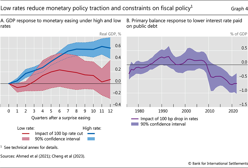
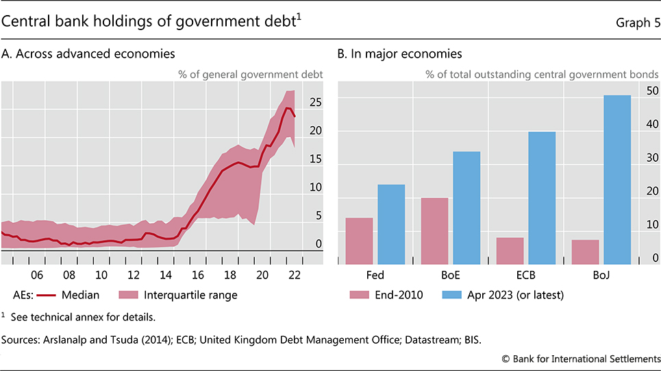
Fiscal stimulus also tends to become less powerful when public debt is higher. This likely reflects adverse confidence effects that kick in when doubts about fiscal sustainability grow. Therefore, larger fiscal measures are required to achieve the same stimulus as debt trends up.10
The self-reinforcing interactions between the two policies constitute a second important factor. Lower interest rates reduced fiscal constraints, diminishing the need and incentive to consolidate in economic expansions. Reductions in the interest rate paid on the debt have indeed been associated with an increase in fiscal deficits, especially during the post-GFC period of ultra-low interest rates (Graph 4.B). Central bank large-scale asset purchases of sovereign debt played a key role in this respect. Across advanced economies, central bank holdings of government debt soared post-GFC (Graph 5.A), driven primarily by large-scale bond purchases of major central banks (Graph 5.B).
High public debt levels, in turn, probably reinforced incentives to maintain an accommodative monetary stance. When debt levels are high, interest rate hikes have a stronger impact on debt servicing costs, raising more acute concerns about adverse macro-financial and fiscal repercussions. By the same token, central bank balance sheet normalisation becomes more difficult when public debt is high because markets must absorb larger amounts of debt. These factors may have made it harder to tighten monetary policy and shrink central bank balance sheets – a kind of “debt trap”.
The journey: how different are EMEs?
The journey of EMEs has several similarities to that of AEs. It was shaped by the same global forces that affected business cycles over time. For one, financial liberalisation – sometimes country-specific – elevated the role of financial cycles and increased the incidence of banking crises. Prominent examples include the Southern Cone crisis in Latin America in the early 1980s, the Tequila crisis in Mexico in 1994 and the Asian crisis of 1997–98. In addition, the globalisation of the real economy weighed on inflation from the 1990s on, reinforcing the impact of the adoption of price stability-oriented monetary policy regimes. These basic similarities are reflected also in the broad evolution of key variables such as inflation, interest rates, fiscal deficits and public debt (Graph 6).
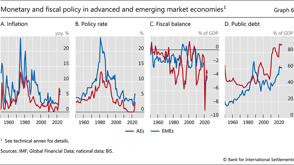
At the same time, there are also important differences, including among EMEs, related to structural factors.
Some of these factors have mainly influenced differences in the journey across EME regions. Political and institutional features can shape attitudes towards fiscal policy, inflation and growth. Partly as a result, inflation has been structurally lower in Asia than in Latin America, which saw hyperinflations in the 1980s and 1990s, often combined with sovereign default and financial stress (Graph 7).11
Other structural factors drive differences, mainly, between EMEs and advanced economies more generally. A key such factor is EMEs’ greater sensitivity to global financial conditions and market sentiment. This greater sensitivity reflects, primarily, less developed financial markets, including fewer FX hedging possibilities, and greater reliance on FX funding.12 It has four main implications.
First, the region of stability is smaller and more fluid. The margin of error is commensurately narrower and the risk of sudden and abrupt discontinuities higher. As a result, when policies step outside the region of stability, market discipline is typically felt earlier and more intensely than in AEs, forcing a rapid shift back.13
Second, the symptoms of breaches of the boundary of the region more often take the form of capital outflows and large depreciations. The exchange rate plays a bigger role, as a force behind fiscal fragility, inflation and financial instability. And given the greater prevalence of fixed or tightly managed exchange rate regimes until the late 1990s, the incidence of currency crises has been higher. This has prompted a shift over time towards more flexible exchange rate arrangements, accompanied by a widespread adoption of inflation targeting frameworks (Graph 8.A).14
Third, the impact of monetary policy in AEs, notably in the United States, given the dominant role of the US dollar, has been especially prominent. Changes in the US monetary policy stance and swings in the US dollar have been major forces behind the ebbs and flows of global conditions. For example, the Volcker disinflation triggered the Latin American debt crisis, characterised by financial fragilities that had been amplified by strong capital inflows linked to the recycling of petrodollars. The shift to more flexible exchange rate regimes has attenuated, but by no means eliminated, this influence.15
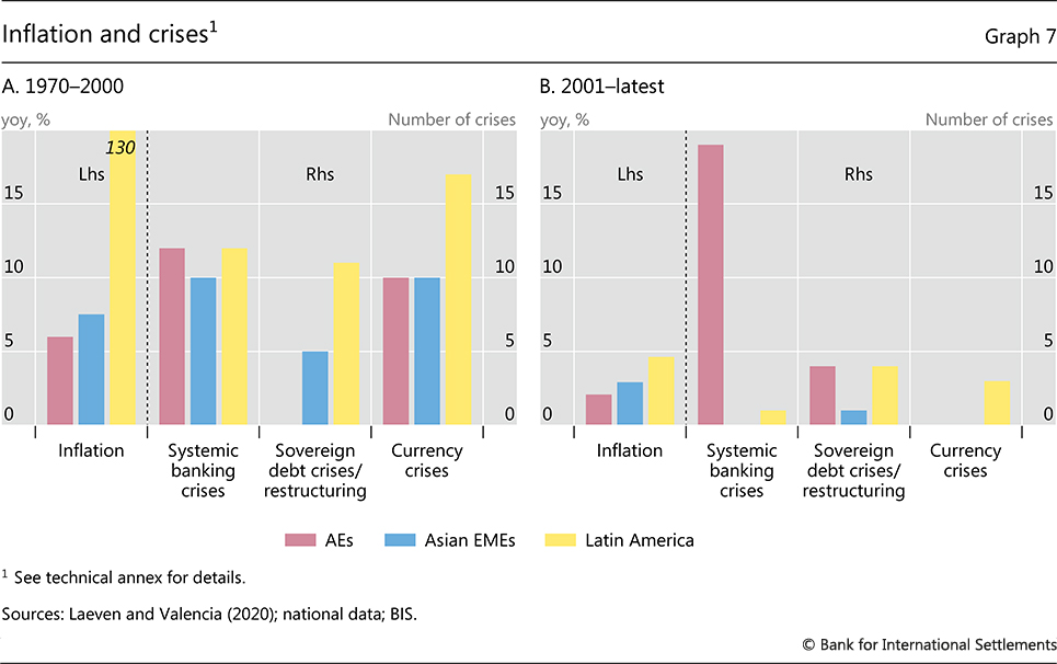
Fourth, the greater exposure to global financial conditions and repeated crises has, over time, fostered EMEs’ awareness of the boundaries of the region of stability and their fluidity. From the late 1990s, well before the GFC, they took steps to strengthen their policy frameworks, complementing flexible inflation targeting with a more active use of FX intervention (Graph 8.B), macroprudential tools (Graph 8.C), as well as, to a lesser extent, targeted capital flow management measures – key elements of macro-financial stability frameworks.16 Again, regional differences emerged, with greater concerns about domestic financial imbalances and a lower degree of exchange rate flexibility in Asia than in Latin America.
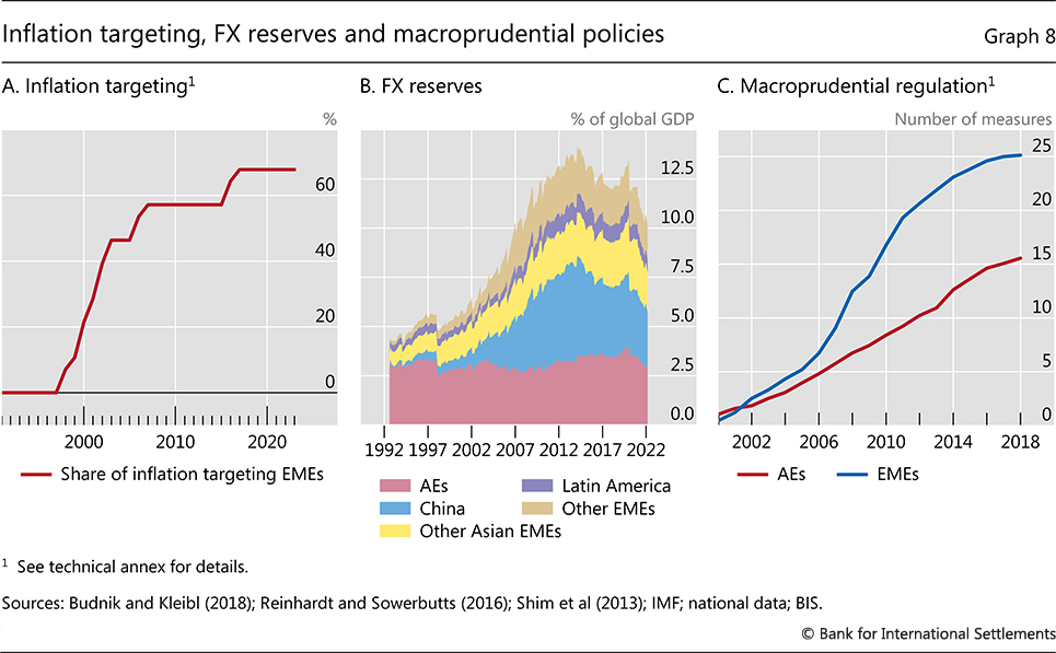
These enhanced policy frameworks have allowed countries to more successfully weather the GFC and the Covid crises (Graph 7) by increasing shock resilience and enabling countercyclical policies in bad times. They also help explain, for example, why countries in Latin America have tightened monetary policy earlier and more forcefully than many of their AE peers post-Covid. At the same time, these improvements have also somewhat relaxed the policy constraints the countries faced, widening the perceived region of stability. This is, in turn, not without risks going forward and could partly account for the deterioration in fiscal positions and ratings post-GFC (see Graph 6 and below).
Testing the boundaries: risks in the journey ahead
What is the next step in the journey of AEs and EMEs? What are the implications of having tested the boundaries of the region of stability? The ongoing struggle to restore price stability and fend off financial stability risks has triggered tensions between fiscal and monetary policy that raise further challenges down the road.
Three main interrelated challenges stand out. First, public finances are facing major strains owing to the combination of record high levels of public debt, strong spending pressures, higher interest rates and weakening growth prospects. Second, large fiscal deficits and high public debt are at risk of working at cross purposes with monetary policy tightening, potentially complicating the fight against inflation. Third, the deterioration in public finances and the sharp repricing of long-term debt in the wake of interest rate hikes may raise financial stability risks.
Consider each issue in turn.
Risks to fiscal positions and the sovereign’s creditworthiness
The increase in public debt in AEs and EMEs has led to a deterioration in sovereigns’ creditworthiness (Graph 9.A). In AEs, sovereign credit ratings worsened considerably following the surge in debt levels in the wake of the GFC. In EMEs, credit ratings have gradually deteriorated during the past decade in line with the increase in debt levels.
The unexpected inflation surge after the Covid-19 pandemic has temporarily embellished fiscal accounts by boosting nominal GDP and thus mechanically reducing debt-to-GDP ratios. Inflation has also flattered fiscal balances. Since many taxes are levied in proportion to nominal variables – such as wages, sales etc – they tend to increase immediately as prices rise. By contrast, public expenditures are largely fixed in nominal terms from year to year.
Yet improvements in fiscal balances due to inflation are ephemeral. Rising costs will feed into higher public spending and governments will confront pressures to raise public wages and social transfers in line with price increases, if this is not already occurring automatically through indexation mechanisms. Furthermore, the monetary tightening required to bring inflation down will increase borrowing costs and constrain economic growth. Indeed, the historical experience shows that periods of higher inflation tend to be followed, if anything, by rising – not declining – public debt (Graph 9.B).
Looking ahead, fiscal authorities will confront severe challenges due to large new spending pressures, the possibility of higher medium-term interest rates and dimmer growth prospects.
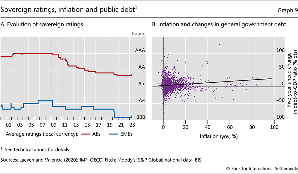
First, consider the implications of new spending pressures for the path of public debt going forward. Estimates for AEs and EMEs suggest that age-related expenditures will grow by approximately 4% and 5% of GDP, respectively, over the next 20 years. Absent fiscal consolidation, this would push debt above 200% and 150% of GDP by 2050 in AEs and EMEs, respectively, even if interest rates remain below growth rates, as was the case in the pre-pandemic years (Graph 10).
Other factors may add to the pressure on public finances. The commitment to supporting a transition towards a sustainable global economy in response to climate change is one. In addition, geopolitical tensions are likely to lead to a material increase in defence spending. An illustrative scenario that includes a rise in public spending by 2% of GDP on top of the increase in age-related spending, would lead to an additional increase in public debt of approximately 50% of GDP by 2050.
These worrying debt projections are, in fact, rather optimistic: they assume that real interest rates will remain 1 percentage point below growth rates, broadly in line with the experience in recent years. As is well known, this configuration tends to ease debt sustainability pressures (Box C).
Indeed, there are two important reasons why it would be imprudent to count on large and permanent negative differentials between interest rates and growth rates. First, inflation may prove stubborn and require higher interest rates for longer than currently expected. High inflation may also lead to a re-assessment of inflation risk, prompting investors to demand higher risk premia to hold government bonds. And attempts to regain price stability may ultimately result in a substantive economic slowdown.
Second, the link between structural factors and low real rates, which is often relied upon to project persistently low interest rates, is not watertight.17 The economy may thus exit the current period of high inflation by confronting a new reality with higher real rates.
Should real rates increase on a sustained basis, public debt sustainability would come under further considerable pressure. Two factors compound the effect of interest rate hikes on public finances.
Box C
Fiscal limits and the risks to debt dynamics
A substantial part of the recent debate on public debt and fiscal sustainability revolves around the idea that a persistently negative differential between the interest paid on public debt and the growth rate of the economy – the so-called interest-growth differential, or, in jargon, r – g – is a boon for public finances. The reason is that it helps preserve debt sustainability irrespective of the fiscal stance. While this is never portrayed as a call for reckless fiscal spending, it does provide some comfort that spare fiscal capacity can be tapped in case of need and encourages more expansionary policies. The degree of comfort, however, can easily be misleading, with material risks.
Historically, a negative interest-growth differential has been relatively common (Graph C1.A). The prolonged period of average positive differentials in advanced economies starting in the 1980s is more of an exception. But the same is true of the relatively low volatility of the differential since the 1990s. Indeed, historically, adjustments in interest-growth differentials have been abrupt and unpredictable.
Textbook approaches to fiscal limits are based on a stylised budget constraint of the narrow government sector and rely on the relationship that outlines the accumulation of public debt (see also Box A):

where Dt is the nominal amount of outstanding debt at time t,rt is the effective interest rate paid on outstanding debt and PBt the primary balance (including central banks’ remittances to the government). Dividing by (nominal) GDP, rearranging terms and approximating, one obtains:

where dt and pbt are, respectively, public debt and the primary balance expressed as a ratio of GDP, and gt is the growth rate of real GDP between t and t – 1. According to equation (2), the dynamics of the debt-to-GDP ratio depend on three key variables: interest rates, nominal growth and net government revenue (the primary balance).
Equation (2) can also be used to determine the adjustment path towards a “long-run” debt level d* from any given starting point and over any time horizon. In the medium run, net of temporary and cyclical factors, rt and gt are assumed to fluctuate around (possibly slowly time-varying) levels r* and g*. The equation can then be solved to determine a long-run value for the debt-stabilising primary balance, that is:

this can be taken as the value around which (countercyclical) fiscal policy should be conducted to maintain debt at the level d*, once cyclical factors have played out.
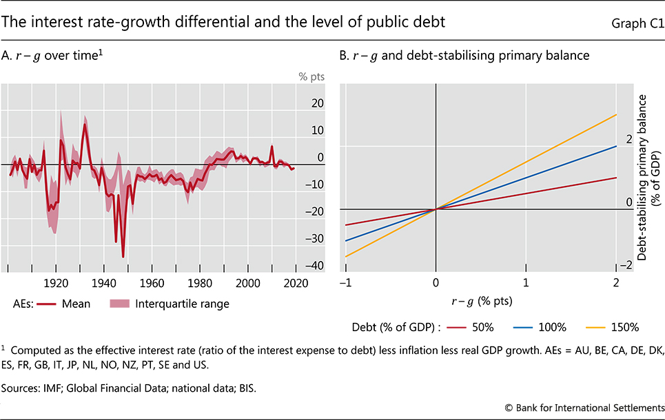
Focusing first on the case r* > g*, higher long-run debt levels require the government to run increasingly high primary surpluses to offset interest payments. But there are limits to running large primary surpluses for extended periods. From a purely economic standpoint, taxes cannot be raised indefinitely without generating incentives to evade taxes, eventually eroding the tax base – the so-called Laffer curve effect. And even more importantly, from a political economy perspective, taxes cannot be raised at will without provoking a backlash, nor can public expenditure be cut below certain limits without jeopardising the provision of basic public services. All these factors imply that there is a limit on the maximum sustainable primary balance, which, together with r* and g*, also establishes an upper limit on public debt – the so-called debt limit.
Keeping in mind the uncertainty of r – g and its sensitivity to the dynamics of debt also helps to avoid the pitfalls of drawing strong inferences from the above stylised identity. It follows that the conclusion that any level of public debt can be sustained when r < g is incorrect. Even if the relationship appears to hold, it does so for a given state of the economic environment, including the level and expected path of public debt: there is no guarantee that r will remain below g once the fiscal stance changes. Uncertainty and endogeneity can, in fact, turn a deceptively safe spot into a situation in which fiscal consolidation is required. Spikes in yields can occur suddenly in response to adverse events, and a high level of indebtedness makes them more likely. Moreover, even if changes in the interest-growth differential are more gradual, the government may find itself constrained in adjusting its fiscal stance. Two factors could get in the way.
The first is a high level of debt. On one hand, this amplifies the reaction of yields to adverse shocks. On the other hand, it magnifies the effects that changes in the interest-growth differential have on the debt-stabilising primary balance. In other words, with higher debt, a given increase in r – g will require a larger adjustment to the primary balance. This is illustrated in Graph C1.B, which shows the relationship between primary balances and debt, as sketched in equation (3). For example, if r increases by 2 percentage points, the necessary increase in the primary balance is just 1 percentage point when debt is 50% of GDP, but it is three times as high when debt is 150% of GDP.
Such a large adjustment may not be feasible due to the political economy constraints mentioned above. And even if technically feasible, investors may question the ability of the government to stick to a painful plan: in the end, their assessment of debt sustainability may rely more on their perceptions of the effective capacity of the sovereign to collect more taxes and/or cut expenditures than on estimates of r – g. This could trigger a credibility crisis and a full-blown run on public debt.
Another source of risk is the maturity structure of the stock of public debt. A comparatively shorter maturity of public debt means higher refinancing needs and a higher sensitivity of rt to changes in market rates. This amplifies the magnitude of sudden increases in the interest-growth differential due to changes in interest rates. Typically, a worsening in sovereign risk goes hand in hand with higher risk premia and a shortening of new bond issuance, as the cost of refinancing at longer horizons is higher. This, in turn, increases rollover risks and makes a run on debt more likely. Furthermore, as fiscal accounts become more sensitive to interest rate changes, this could hamper the ability of monetary policy to control inflation.
In practice, estimating the debt limit is a daunting task. First of all, it is unclear where one should place the limit on primary balances. Historical experience suggests that primary surpluses are unlikely to exceed 5% for extended periods. Yet country- and episode-specific circumstances can play a large role in determining such a threshold, which should be taken with a pinch of salt. Second, there is considerable uncertainty about the possible evolution of future interest rates and GDP growth rates. Finally, and more importantly, they are also likely to be interrelated and endogenous to debt itself. Higher indebtedness is likely to be associated with higher risk premia, and hence higher interest rates to be paid on public debt. Moreover, there is some evidence that high public debt can be associated with lower growth. Accordingly, the only reasonable approach to gauging fiscal limits is to use stress tests or to compare the effects of alternative assumptions.
All in all, running public finances in a region that is closer to the limits increases the risk of abrupt adjustments that could derail the economy. A prudent approach is called for.
See eg Blanchard (2019). However, recent research argues that what matters for the sustainability of public debt is not only the interest-growth differential, but also the difference between the marginal product of capital and the growth rate of the economy, see eg Reis (2021). One possible reason is that, when creditworthiness is preserved, public debt can provide investors with liquidity and safety, and hence trades at a premium over other riskier and less liquid assets. See also Mauro and Zhou (2021). For example, Mian et al (2022) argue that the debt sustainability condition needs to be explicitly complemented by a term accounting for the sensitivity of interest rates to the debt level. For example, Lian et al (2020) show that the probability and the size of reversals in r – g are related to the size of public debt and the share of foreign currency debt. Note that a similar scenario could be one in which inflation surges and the central bank struggles to control it. See Eichengreen and Panizza (2016). Threshold effects of debt on growth are also used by IMF (2018).
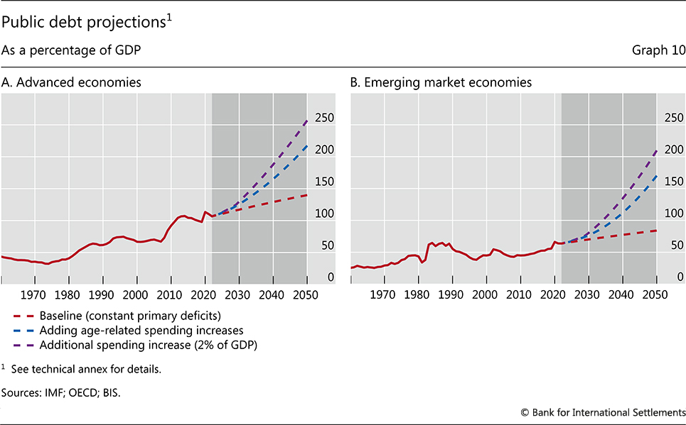
The first is the post-GFC large-scale government bond purchases implemented by several central banks. These purchases – which amounted to 25–50% of the outstanding stock in major AEs (Graph 5.B) – were financed with central bank reserves, thus shortening the maturity of the consolidated public debt. This implies that higher interest rates transmit much faster to public finances via reduced remittances from central banks. Indeed, after accounting for approximately 6% of interest payments on public debt in 2010–20, central bank transfers to governments in AEs have already declined to zero in most countries (Graph 11.A).
The second, much more general factor is the historically high levels of public debt, which means that higher interest rates can lead to a large increase in debt service costs. For example, should interest rates return to levels prevailing in the mid-1990s, interest rate payments on public debt would, over time, surge above 6% of GDP – the highest level in the post-World War II period (Graph 11.B).
Pressures on public debt would increase further should medium-term growth prove disappointing. Global growth prospects are the weakest in decades owing to several structural forces, including geoeconomic fragmentation, slower labour force growth, and slowdowns in China and other EMEs.18 In addition, risks to fiscal positions may themselves weaken economic prospects and raise the risk of adverse non-linear effects. For example, high public debt may constrain the ability of fiscal policy to operate countercyclically during recessions. This could erode confidence in the economic outlook, thus reducing private investment and growth. In turn, weaker growth prospects may exacerbate fiscal risks, increasing risk premia and further undermining economic activity. Countries with higher public debt levels thus tend to experience shorter phases with interest rates lower than growth rates, as well as a higher probability of a reversal.19
In EMEs, the potential for vicious circles between fiscal sustainability, slowing growth and rising interest rates is higher. One key reason is that exchange rate reactions can suddenly push countries to bump up against debt limits. Loss of confidence in debt sustainability can trigger sharp depreciations that, in the presence of currency mismatches can wreak havoc on public and private balance sheets, leading to exploding debt service costs and severe recessions.
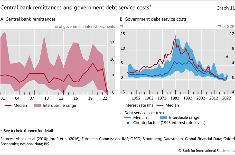
Inflation risks
Pressure on fiscal positions and sovereign risk may increase inflation risks going forward.
In the near term, fiscal deficits remain large in many countries, thus sustaining aggregate demand and inflation. Hence, monetary and fiscal policy are at risk of working at cross purposes, complicating the fight against inflation (Chapter I). This heightens the risk of transitioning to a high-inflation regime – a concern that becomes more acute the longer inflation remains elevated.
Taking a long-term perspective sheds further light on these risks. The evidence indicates that the inflationary effects of fiscal policy depend on the fiscal and monetary policy regime. In AEs, if fiscal policy is prudent – leaning against public debt increases through higher primary balances – and central banks are independent, fiscal stimulus has modest effects on inflation (Graph 12.A).20 But if fiscal policy fails to stabilise debt (ie is profligate) and central bank independence is questioned, the inflationary effects of fiscal policy are much stronger.
The effects of fiscal stimulus on inflation tend to be greater in EMEs (Graph 12.B). This is largely due to the role of the exchange rate. In advanced economies, fiscal stimulus tends to have no significant effect on the exchange rate. By contrast, fiscal expansions in EMEs trigger a significant depreciation of the exchange rate.21 In turn, exchange rate depreciations feed into higher inflation, and to a larger extent than in advanced economies (Graph 13.A).
The transmission of fiscal stimulus to exchange rates in EMEs largely reflects concerns about sovereign risks. Fiscal expansions are associated with increases in sovereign risks, as captured by credit default swap (CDS) spreads (Graph 13.B). These increases, in turn, trigger depreciations (Graph 13.C). In this respect, exchange rates act as the proverbial canary in the coal mine, being highly responsive to the first signs of macroeconomic instability. Beyond feeding back into higher domestic prices and thus undermining efforts to contain inflation, exchange rate depreciations can also pose considerable financial stability concerns.
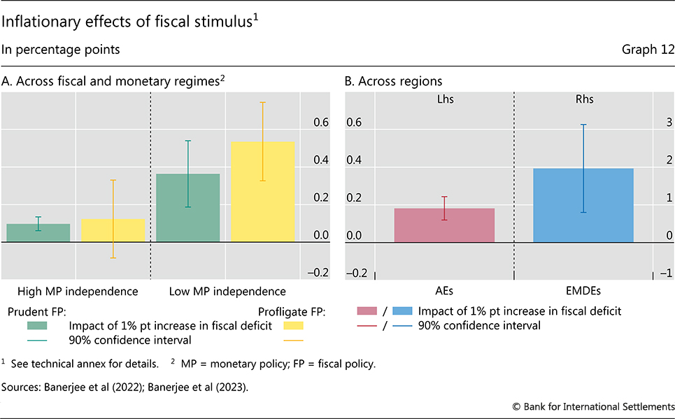
Beyond the impact of fiscal deficits on inflation, high levels of debt may also play a role by constraining the room for manoeuvre of monetary policy. The most acute concern is the risk of fiscal dominance, ie a situation in which monetary policy is unable to tighten due to fiscal constraints (see also Box A).22 Fiscal dominance can arise for two reasons. In some cases, the central bank is subject to political economy pressures to expand fiscal space by keeping interest rates low. In other circumstances, monetary policy faces an economic constraint because interest rate hikes risk precipitating a sovereign debt crisis.
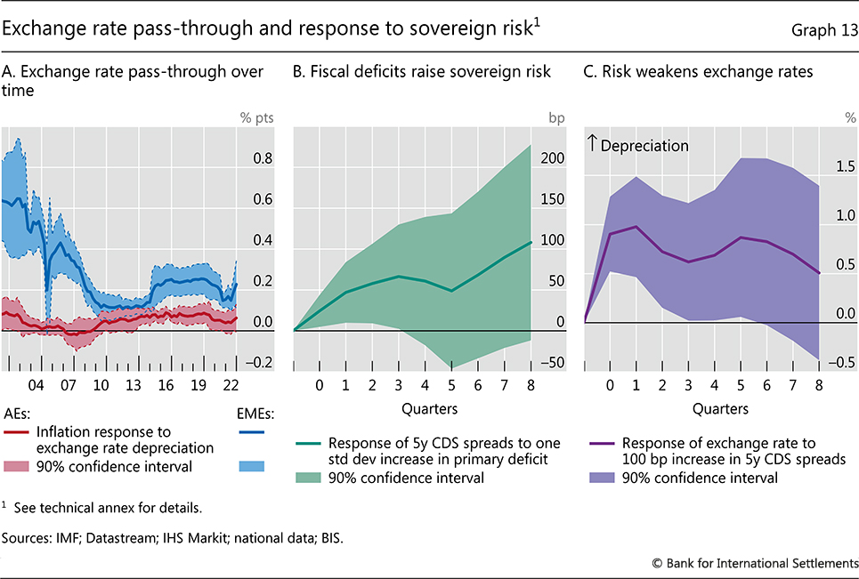
While the two types of dominance tend to go hand in hand and can undermine the central bank’s credibility and independence, they have somewhat different implications. Strong institutional safeguards designed to shield the central bank’s operational autonomy can be effective when pressures are purely of a political nature. By contrast, they can do relatively little when the constraint is economic and reflects trade-offs linked to higher rates.
Even if high debt levels do not lead to outright forms of fiscal dominance, they may still contribute to raising inflationary pressures. For example, survey evidence suggests that high public debt increases household inflation expectations, especially among people that have less confidence in the central bank’s determination to fight inflation.23
Financial stability risks
The deteriorating sovereign debt outlook in many economies also points to heightened risks for the financial sector. Ultimately, a vulnerable sovereign means a vulnerable financial system. There are two reasons for this, over and above any negative effects on the financial system generated by adverse macroeconomic outcomes.
The first reason is that, most directly, the financial system is exposed to the sovereign. To be sure, sovereign debt can be a cornerstone of a well functioning financial system. It can underpin the system’s smooth functioning, by providing a safe store of value, a solid benchmark for the pricing of assets and a liquid asset that facilitates economic transactions, not least in its role as collateral (eg for repos or to meet margin calls; Box D). Moreover, government debt is a key instrument through which the central bank sets interest rates and implements monetary policy. At the same time, for government debt to fulfil such functions effectively, it is essential that it retains the highest credit quality and that financial institutions manage the associated interest rate risks properly. Otherwise, it can easily turn from a source of stability into one of major instability.
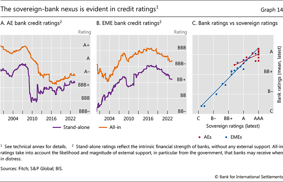
Box D
Government debt as collateral and market functioning
Government debt plays a key role in the financial system. It is typically the domestic currency asset with the highest credit quality. It is traded in the deepest and most liquid markets, and provides the benchmark for pricing virtually all other assets. It is the main instrument that central banks use in their liquidity management operations to set policy interest rates or, through large-scale asset purchases, to influence asset prices more broadly. And, increasingly, it is a primary form of collateral.
The use of government securities as collateral, broadly defined, is an integral part of market participants’ risk management and underpins vast financial markets. Government paper is extensively used to post margins in derivatives transactions to reduce counterparty credit risk (Graphs D1.A and D1.B). And it is the instrument of choice in repurchase agreement (repo) transactions (Graph D1.C), which involve the exchange of securities for cash for a pre-defined period. Repos are functionally equivalent to borrowing/lending against collateral.
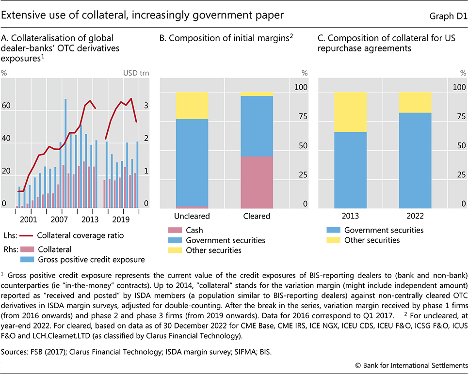
Several reasons explain the use of government debt as collateral. First, policymakers’ objective of boosting the depth and liquidity of government bond markets was a key motivation behind the development of repo markets. Second, lenders’ preferences to substitute relationship finance with arm’s length finance naturally shift the focus from the creditworthiness of the counterparty or borrower to the quality of the asset used as collateral. Third, post-GFC regulatory and financial system reforms have incentivised the use of collateral as an additional risk mitigant.
Government paper has thus acquired the status of “quasi-money”. It competes with cash – mostly bank deposits or bank reserves with the central bank – in derivatives margins (Graph D1.B). And, through repos, holders can raise cash without having to sell the underlying security. In fact, haircuts in core safe government bond markets are often tiny or non-existent, in the range of 0–2%. This means that an investor can raise almost as much cash as the value of the government paper they hold.
This quasi-money property of government paper puts a premium on it retaining the highest credit quality. Conversely, deteriorating perceptions about sovereign credit risk and the attendant rise in haircuts can generate major market dislocations, as was evident during the euro area sovereign debt crisis. But, even short of that happening, the pervasive use of government paper as collateral can have major implications for the dynamics of markets under stress.
One reason is rooted in the system’s procyclicality. In good times, the availability of collateral and compressed margins can contribute to the build-up of vulnerabilities. As leverage and liquidity mismatches expand, the perceived need to screen and monitor the creditworthiness of counterparties declines, thus leading to a build-up of credit risk, paradoxically when risks seem particularly low on the surface. In bad times, as risk materialises and/or market volatility picks up, spikes in haircuts and margins put a premium on the safest and most liquid forms of collateral, such as government paper. This can set in motion fire sales of less liquid assets to satisfy collateral needs. In the extreme, liquidity strains can degenerate into outright solvency concerns.
A second reason is that, while the use of government paper as collateral may be compelling at the level of each individual agent, widespread use may ultimately undermine this paper’s safe haven status and generate systemic events. A certain “fallacy of composition” would be at work, whereby an initial decline in the value of collateral induces many market participants to sell it at the same time, thus giving rise to destabilising price dynamics. One possible trigger is an unexpected tightening of monetary policy. This is what occurred, for instance, during the bond market crash of 1994, when highly leveraged positions in government paper were unwound. Another possible trigger is escalating concerns about inflation. Such concerns appeared to play a role in the recent stress in UK gilt markets. Following a fiscal announcement that pointed to a highly expansionary stance, government paper was sold and the drop in its price was amplified by the deleveraging of investment vehicles on which pension funds had been relying to hedge the duration risk of their liabilities.
The potential for unintended consequences of widespread collateral use carries policy messages. In particular, there is a strong case for imposing higher collateral haircuts and margins that limit the increase in leverage during good times and dampen the ensuing contraction in bad times. While such measures to contain procyclicality would still exploit the risk-mitigating properties of collateral, they would reduce the likelihood of liquidity shortages or declines in collateral values that necessitate central bank interventions.
See for instance CGFS (1999). BCBS (2013, 2020), BCBS-IOSCO (2020) and FSB (2017). See also Aramonte et al (2022). Borio and McCauley (1996). Aramonte and Rungcharoenkitkul (2022).
Historically, the spectre of a loss of sovereign creditworthiness has been a major source of risk for the financial system. In the extreme, the sovereign can default on its debt, causing large losses for debt holders.24 Even in the absence of default, a serious erosion of sovereign creditworthiness can trigger stress and higher risk premia in the government bond market. This propagates to banks, other financial institutions and capital markets, weakening balance sheets and tightening funding conditions, possibly even precipitating a crisis.
The second reason why a vulnerable sovereign can threaten the financial system is that the government provides the ultimate backstop for the system. Of course, prudential regulation and strong standalone resolution mechanisms are the first line of defence. Moreover, central banks can act as lender of last resort and market-maker of last resort in times of severe stress, thereby buttressing the liquidity of the system. But only the government can backstop the system’s solvency, through deposit insurance and other guarantees, as well as, when needed, outright recapitalisation of failing institutions.25
This backstop role is visible in bank ratings. The fact that banks’ all-in credit ratings are meaningfully above their stand-alone ratings highlights the importance of implicit government guarantees (Graph 14.A).26 The wider ratings gap for EMEs compared with AEs suggests that reliance on the creditworthiness of the sovereign – and the potential cost for the government – are particularly important for EME banking systems (Graph 14.B).
Indeed, partly because of the sovereign’s backstop function, the fiscal costs (direct and indirect) of financial crises are typically huge, as measured by the change in public debt following a crisis. Historically, public debt has tended to jump in the aftermath of a banking crisis, in both AEs and EMEs (Graph 15). The fiscal cost was especially large in the case of the GFC, reaching a median rise in debt-to-GDP of about 40 percentage points in AEs. A significant portion of crisis costs typically reflect fiscal recapitalisation packages and other outright support for the banking sector, although the bulk represents indirect costs from the macroeconomic fallout and any discretionary fiscal responses.27
The two-way link between the sovereign and the financial sector gives rise to the risk of a costly feedback loop. Through it, deteriorations in the creditworthiness of the sovereign and the banks can reinforce each other – the proverbial doom loop of the sovereign-bank nexus.28 Such episodes have been more common in EMEs. But the sovereign debt crisis in the euro area has shown that AEs are not immune.29 Credit ratings show that the credit risk of sovereigns and banks are tightly connected in both EMEs and AEs (Graph 14.C). Similarly, spreads on CDS referencing sovereign assets and bank assets are typically tightly linked, indicating that bank and sovereign risks tend to move in tandem.30
Over the past decade, the rapid increase in sovereign debt has left investors and financial intermediaries increasingly exposed not only to sovereign credit risk, but also to interest rate risk.31 This is particularly the case, as governments increasingly issued longer-maturity debt during the low-yield era to lock in low financing costs (Graph 16.A). And even though large-scale asset purchases by some AE central banks reduced exposures by replacing sovereign debt with bank reserves in private sector portfolios, the average maturity of debt net of central bank purchases has still risen since pre-GFC (Graph 16.B). A hypothetical 300 basis point increase in government bond yields, for example, would result in estimated losses to bondholders (excluding the central bank) corresponding to between approximately 10 and 35% of GDP in major AEs, and up to 10% in major EMEs (Graph 16.C). Those losses would have been even larger had it not been for central banks’ asset purchases, especially among AEs.
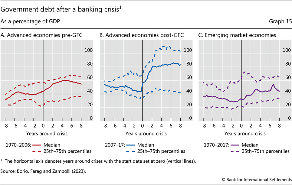
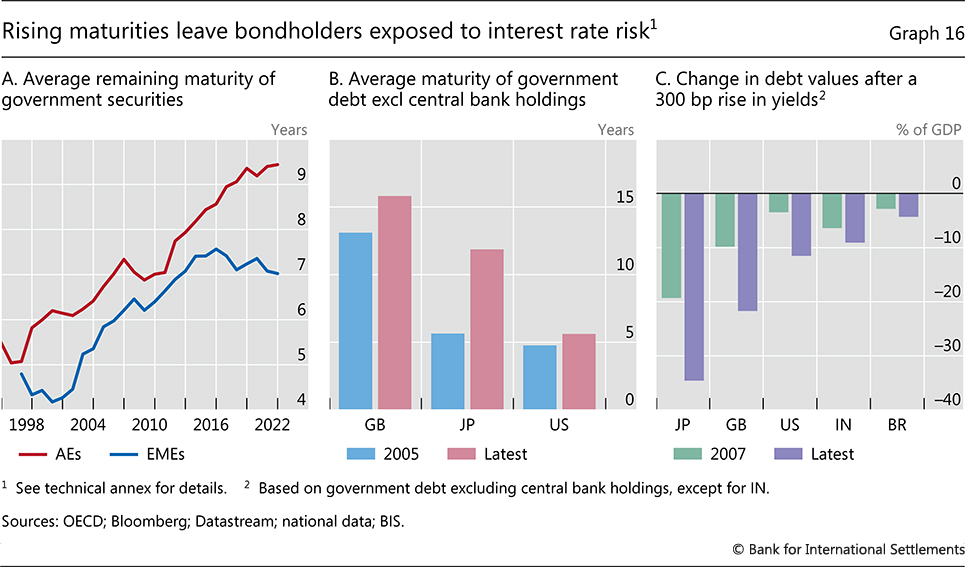
Within the financial sector, banks and NBFIs were the main investors in government securities. Banks across advanced and emerging market economies hold large quantities of sovereign bonds, in some cases multiple times their capital (Graph 17.A and 17.B). NBFIs have been playing an increasing role, following their rapid growth post-GFC. The sector, which holds close to half of total financial assets globally,32 on average accounts for approximately 40% of government bond holdings in AEs and 60% in EMEs.33 The tight interconnections between banks and NBFIs mean that distress can easily spread between the two sectors and intensify in the process (Graph 17.C).34
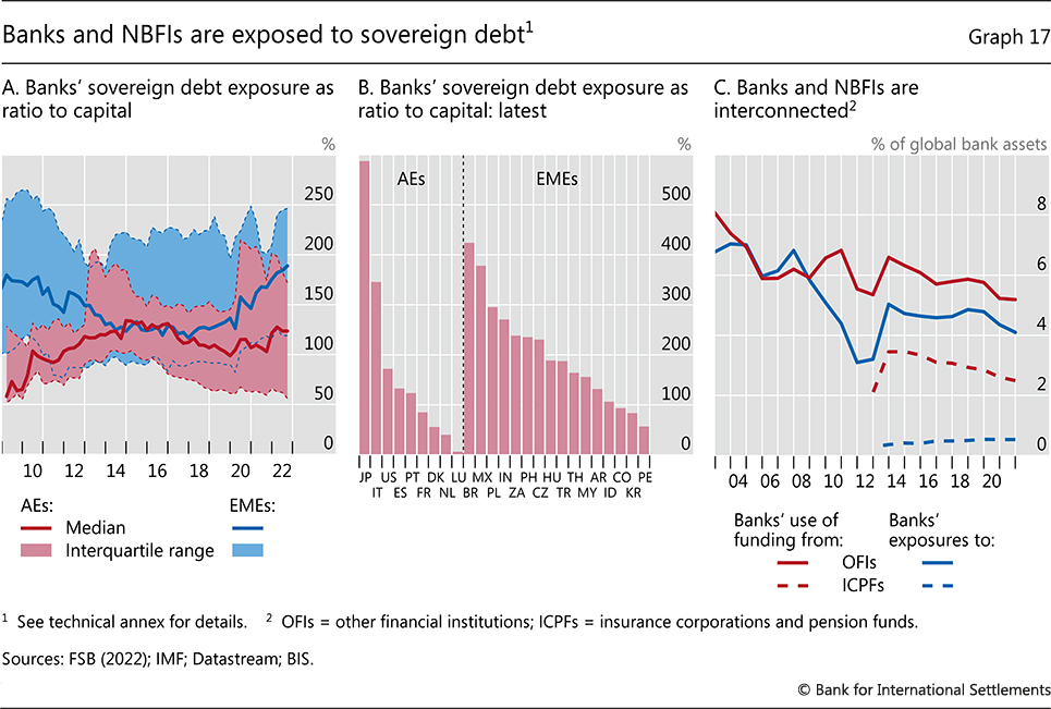
High sovereign debt heightens the risk to the financial system not just because of the sheer size of the exposures but, importantly, because it increases the likelihood of sharp bond yield moves. In particular, during monetary policy tightening phases, long-term yields have tended to rise more in high-debt countries than in low-debt countries, especially among EMEs (Graph 18.A). To a significant degree, this has been due to higher credit risk premia: sovereign CDS premia have tended to rise markedly for high-debt EMEs when monetary policy is tightened, but not for low-debt EMEs (Graph 18.B). While the effects of rate hikes on yields are smaller for AEs, this is based on a sample that includes a prolonged period of heavy government debt purchases by AE central banks. As these purchases end and begin to reverse, the situation may change.
The risk of sharp yield adjustments is higher when liquidity in bond markets is structurally poor. The Covid-19 crisis showed how quickly market functioning can break down when liquidity conditions in sovereign bond markets are fragile. In March 2020, one-sided selling pressure (the “dash for cash”) – disorderly deleveraging by hedge funds and other players – interacted with intermediation bottlenecks to create a perfect storm that led to dysfunction even in markets that are typically among the most liquid ones in the world.35 The fact that, currently, indicators point to fragile liquidity conditions suggests that risks of market dysfunction should not be underestimated (Graph 18.C).
One factor that has amplified the impact of government debt on market dynamics under stress is its pervasive role as collateral (Box D). On the one hand, this allows greater build-up in leverage. On the other hand, it intensifies fire sales when the system is hit by shocks that induce agents to sell the paper. This can undermine the safe haven status of government bonds even when their credit quality is not in doubt.
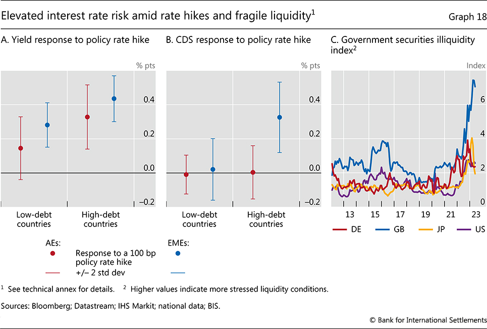
In the current hiking cycle, government debt exposures have already been a source of financial stress. So far, the problems have been linked to interest rate risk, not sovereign risk (Chapter I). They have reflected the accumulation of exposures during the long phase of unusually low interest rates. Losses on government bond holdings have been at the heart of recent stress in the banking system in the United States and of NBFIs in the United Kingdom. The stress has prompted broad-based central bank liquidity support and, in the case of the banks, the extension of deposit guarantees, which in turn increases the potential costs to public finances. Looking ahead, however, given prospective further deterioration in the creditworthiness of sovereigns, credit risk could also become, once again, a source of stress.
This analysis suggests that the financial sector is especially vulnerable following a prolonged period of lax fiscal policy and loose monetary policy. This is because the overall size of sovereign exposures is higher, the sensitivity of those exposures to adjustments in yields is greater and the likelihood of those adjustments is also greater. If investors perceive that the policy mix is reaching the boundaries of the region of stability, government bonds could reprice rapidly and forcefully. Yields would rise sharply as investors would require significantly higher compensation to be exposed to inflation risk or, especially in the case of EMEs, to sovereign credit risk. And sovereigns with lower creditworthiness would be particularly vulnerable. This, in turn, would compound risks among banks and other financial institutions.
Policy implications
The analysis of the journey to the boundaries of the region of stability and of the risks ahead raises both near- and longer-term challenges for monetary and fiscal policy.
In the near term, the challenge is to ensure a consistent policy mix that delivers a return to low inflation while tackling financial stability risks (Chapter I), thereby withdrawing from the boundaries of the region of stability. The priority for monetary policy is to restore price stability. Should a shift to a high-inflation regime take place and inflation become entrenched, it would be very costly to return to a regime of low and stable inflation.36 At the same time, monetary policy will have to alleviate financial strains to prevent systemic financial instability. There will be a premium on distinguishing, to the extent possible, the measures designed to achieve the two objectives. Regardless, it will be essential to ensure that the tightening path consistent with lower inflation is not compromised by the immediate needs of the financial sector. Fiscal policy plays an important complementary role. Through consolidation, it would help to reduce pressure on aggregate demand and inflation, limit the risk of being a source of financial instability and provide more headroom, should it be called upon, to support crisis management by tackling solvency concerns.
The longer-term challenge is to ensure that monetary and fiscal policies operate well within the region of stability on a lasting basis, heeding the lessons learnt along the journey. This has implications for strategies, institutions and mindsets.
To avoid testing the boundaries of the region of stability, policy strategies should aim to retain room for policy manoeuvre over time. In the journey to the boundaries over the past decades, these safety margins evaporated to a significant extent due to an asymmetric conduct of policy over the business cycle, with easing in the bust not compensated for by a commensurate tightening in the boom.
To retain greater monetary space, once price stability is re-established, monetary policy could be more tolerant of moderate, even if persistent, shortfalls of inflation from point targets. In a low-inflation regime, inflation has certain self-stabilising properties, so that there is less need to respond forcefully to correct deviations from target. Furthermore, the evidence indicates that monetary policy has less traction in lifting inflation under such conditions. Such a refinement in frameworks would also help limit the side effects that arise from prolonged periods of monetary accommodation. Foremost among such side effects is the build-up of financial vulnerabilities, which tend to further constrain both monetary and fiscal policy headroom when financial stress emerges.
Careful consideration should also be given to keeping central bank balance sheets as small and as riskless as possible, subject to delivering successfully on the mandate. This would have three benefits. First, it would limit the footprint of the central bank in the economy, thereby reducing the institution’s involvement in resource allocation and the risk of inhibiting market functioning. Second, it would lessen the economic and political economy problems linked to transfers to the government. Finally, it would maximise the central bank’s ability to expand the balance sheet when the need does arise. Given the costs of large and risky balance sheets, the initial size is a hindrance, not an advantage. The balance sheet needs to be elastic, not large.
As for fiscal policy, there is an urgent need to consolidate fiscal positions. Relying on inflation to reduce the government debt burden is obviously not an option. It would have only a temporary effect. And, in the longer run, it would generate the very instability that would seriously damage the economy and public finances in the process. Moreover, to support consolidation it would be useful to incorporate the role of financial factors more systematically. For instance, when assessing fiscal space, it would be important to account for the flattering effect of financial booms on fiscal accounts and the possible costs of financial stress. Greater reliance on automatic stabilisers more generally would also help.
Consolidation should go hand in hand with fiscal strategies that boost sustainable growth. For one, efforts could be made to reduce or eliminate the typical bias in tax systems that favours debt over equity. This has encouraged excessive reliance on debt as an engine of growth. In addition, the quality of public spending is crucial. For example, it would be important to rebalance government expenditures towards well chosen and effectively executed investment projects – especially in infrastructure and green energy – as well as human capital building (education and health). Such a rebalancing would correct a decade-long downward trend in public investment that made room for more inflexible spending components, such as entitlements. Quite apart from being an ultimate policy objective, higher growth would also deliver stronger public finances and at higher real interest rates – more in line with an efficient allocation of capital and resources.
Beyond adjustments to monetary and fiscal policy strategies, institutional safeguards are necessary to limit tensions between the two policies and promote their coherence. Central bank independence remains the key pillar to ensure that monetary policy can pursue its price stability mandate, especially in the current context of elevated public debt levels and stubbornly high inflation. On the fiscal side, stronger institutional safeguards would help encourage prudent fiscal policy. To this end, fiscal rules and fiscal councils could play an important role in setting guardrails, all the more so if backed by appropriate constitutional provisions.
But policy adjustments should not be limited to monetary and fiscal policy alone. Other policies can play a complementary role.
Prudential policy is critical, given how disruptive financial instability can be for the region of stability. Both its microprudential and macroprudential dimensions are important.
As regards microprudential regulation and supervision, a lot has been done following the GFC. That said, progress has been uneven. And recent strains in the banking sector indicate that there is still work to do, with respect to both regulatory standards and, equally importantly, supervisory practices (see Chapter I for an elaboration). Some of that work relates more specifically to the risks linked to sovereign exposures. For banks, the Basel III framework continues to apply a preferential regulatory treatment to those exposures, particularly with regard to credit/default, interest rate and liquidity risks for exposures valued at amortised cost and held in the banking book.37 Similarly, while efforts are under way to address NBFI vulnerabilities, these have so far been insufficient, including with regard to the NBFI-sovereign nexus. As such, more could be done to ensure that regulation better mitigates sovereign risk for both banks and NBFI entities and to avoid undue risk concentrations.38 Any such stricter prudential treatment would need to be calibrated and implemented in the light of the special role of sovereign debt in the financial system.
Macroprudential regulation is an important complement to its microprudential counterpart. Well calibrated, it can help deal with, and mitigate, the costs and intensity of domestic financial cycles.39 It can also help address the consequences of ebbs and flows of global financial conditions, supported by foreign exchange intervention and, in case of need, capital flow management measures.
The ultimate objective would be to set up a more holistic macro-financial stability framework. In such a framework, monetary, fiscal and prudential policy would operate in a coherent fashion to foster economic stability. This would considerably alleviate trade-offs and avoid overburdening individual policies. Post-GFC, major steps have been taken in that direction. That said, this is still very much a work in progress, analytically and practically.40 And the integration of fiscal policy has not proceeded as far as the others.
Sound structural policies boosting sustainable growth will be key to relieve monetary and fiscal policy from the pressures to act as engines of growth which pushed them beyond the boundaries of the region of stability. Achieving higher and sustainable growth can only be accomplished by boosting the productive potential of the economy through effective measures that enhance the supply side. Over the past decades there has been a worrying slowdown in global growth. The slowdown was driven, in particular, by a marked decline in the growth of total factor productivity (TFP), which measures the efficiency of use of labour and capital inputs. To revive TFP growth, therefore, it is essential to enhance the efficiency of production. This requires renewed efforts to design and implement structural reforms, which have slowed substantially since the early 2000s. Boosting competition in product markets, reducing red tape and facilitating a more efficient allocation of labour are key areas to provide new impetus for innovation and growth.
Ultimately, what is needed is a change in mindsets. Policymakers need to have a keener recognition of the limitations of macroeconomic stabilisation policies. Monetary and fiscal policy can be a major force for good, but, if overly ambitious, can also cause great damage. The journey described in this chapter shows that, if the specific challenges evolve with the economic landscape, the root cause of failures does not. The fallacies of the “growth illusion” highlight that stabilisation policies cannot be engines of lasting economic growth.41 The concept of the region of stability, hard as it may be to apply in real time, can promote the necessary shift in perspective. This is because the concept embodies the recognition of the limitations of macroeconomic policies. The region is first and foremost not a precise set of numbers, but a lens through which to look at the world and to guide policy. It can help preserve the all-important trust that society must have in the state and its decision-making.
Endnotes
1 See Carstens (2023).
2 See Carstens (2022).
3 The concept of a region or corridor of stability was coined by Leijonhufvud (2009) in the early 1970s to indicate how the economy can become unstable if it is operating outside a particular range. Borio and Disyatat (2021) have underscored how this region places constraints on the room for manoeuvre for fiscal and monetary policy while in turn being affected by the cumulative fiscal and monetary stance over time.
4 See Padoa-Schioppa and Saccomanni (1994).
5 See Aikman et al (2022).
6 For empirical estimates of the flattering effects of financial booms on fiscal balances, see Borio et al (2017).
7 See BIS (2022a) for a detailed analysis.
8 See Ahmed et al (2021). In addition, changes in the policy stance appear to have a smaller effect on inflation in low-inflation regimes. This is because, as one might expect, monetary policy has a larger impact on the common component of price changes – a measure closer to the concept of “true” inflation – than on relative price changes, see BIS (2022a) and Borio, Lombardi, Yetman and Zakrajšek (2023).
9 This effect is reinforced by larger effects of a given change in the monetary policy stance on asset prices and credit over time, see BIS (2015) and Hofmann and Peersman (2017).
10 For evidence on the negative link between fiscal multipliers and the level of public debt, see Ilzetzki et al (2013) and Banerjee and Zampolli (2019).
11 For a discussion of the roots of inflation in Latin America, see Bernanke (2005). Kehoe and Nicolini (2021) provide a detailed account of the monetary and fiscal interactions in Latin American countries since the 1960s.
12 See BIS (2019, 2022b) and CGFS (2019).
13 For instance, as a result of a history of inflation and default, the safe level of external debt can be very low for many EMEs due to the “debt intolerance” of investors (Reinhart et al (2003)).
14 As highlighted by Calvo and Reinhart (2002), there is often a discrepancy between de jure and de facto exchange rate regimes. In particular, many EMEs have flexible exchange rate regimes officially, but in practice pursue managed exchange rate arrangements limiting exchange rate swings and reflecting the vulnerability to such swings.
15 See BIS (2019, 2020, 2021, 2022b) for analyses of the enduring challenges of capital flow and exchange rate fluctuations for policy frameworks in EMEs.
16 For a discussion of the features of EME macro-financial stability frameworks, see BIS (2019, 2022b).
17 Empirical analyses examining the historical relationship between real interest rates and the standard set of saving-investment drivers find – without imposing strong theoretical priors – little evidence of a systematic link; see eg Borio et al (2017) and references therein.
18 See IMF (2023).
19 These facts are documented in Lian et al (2020) based on a large panel of advanced and emerging market economies since 1950. See also Mauro and Zhou (2021) for evidence that negative differentials between interest rates and growth rates are not systematically associated historically with a lower risk of government default.
20 The classification of fiscal regimes as prudent or profligate follows Mauro et al (2015).
21 See Banerjee et al (2023).
22 The classical statement of fiscal dominance goes back to Sargent and Wallace (1981).
23 Grigoli and Sandri (2023) examine the sensitivity of household inflation expectations to public debt levels using information provision experiments in surveys conducted in Brazil, the United Kingdom and the United States.
24 Sovereign loss-given-default rates have averaged 37% based on a sample of 180 defaults in 68 countries over the period 1970 to 2010; see Cruces and Trebesch (2013).
25 Moreover, to the extent that the sovereign supports the broad economy, it reduces defaults and unemployment, and hence supports the financial system.
26 Stand-alone ratings reflect the intrinsic financial strength of banks, ie the likelihood of default provided that no external support is forthcoming. All-in ratings take into account the likelihood and magnitude of extraordinary external support, in particular from the government, that banks may receive when in distress. See Packer and Tarashev (2011) for a discussion.
27 For banking crises in AEs, the direct fiscal costs related to financial sector support corresponded, on average, to approximately a third of the total increase in public debt following the crisis. Taking into account any subsequent recoveries, the ratio was around one fifth. See Laeven and Valencia (2013, 2018) for details.
28 See eg Farhi and Tirole (2018) and Borio, Farag and Zampolli (2023).
29 See eg Li and Zinna (2018).
30 See the discussion in Borio, Farag and Zampolli (2023) and references therein. Dieckmann and Plank (2012) analyse the sovereign CDS market in AEs and find evidence of a private-to-public risk transfer through expectations of government bailouts.
31 See eg English et al (2018).
32 See FSB (2022).
33 The figure for AEs excludes the United States, where NBFIs hold around 60% of government bonds, and the figure for EMEs excludes China, for which the share is about 40%. See Fang et al (2022).
34 See also BCBS (2022).
35 See Schrimpf et al (2020), Eren and Wooldridge (2021) and FSB (2022).
36 See BIS (2022a) and Borio, Lombardi, Yetman and Zakrajšek (2023).
37 See BCBS (2017).
38 See Borio, Farag and Zampolli (2023).
39 See BIS (2018).
40 See BIS (2022b).
41 See Carstens (2022).
Technical annex
Graph 1: Statistics are computed using a smaller set of countries when data are not available.
Graph 1.A: The sample covers AR, AU, BE, BR, CA, CH, CL, CN, DE, ES, FI, FR, GB, HK, ID, IE, IN, IT, JP, KR, MX, MY, NL, NO, PE, PH, SE, SG, TH and US.
Graph 1.B: General (if not available, central) government core (if not available, total) debt at nominal (if not available, market) value. The sample covers AR, AT, AU, BE, BR, CA, CH, CL, DE, DK, ES, FR, GB, GR, IN, IT, JP, NL, NO, NZ, PT, RU, SE and US.
Graph 2.A: Inflation measured as year-on-year growth rate; mean across countries in sample: AR, BO, BR, MX, PE, UY and VE. Central bank claims on government is the sum of claims on central, state and local government, and public non-financial companies.
Graph 3: Business cycle dates are from National Bureau of Economic Research for US; Economic Cycle Research Institute for AU, CA, CH, DE, ES, FR, GB, IT, JP and SE. For BE, FI, IE, NL and NO business cycles are dated with a business cycle-dating algorithm. Episodes for which data for the previous and next 20 quarters are available are used in computing the medians.
Graph 4.A: Impulse response of real GDP to a 100 bp expansionary monetary policy shock. The threshold for the low rate regime is 2.25%, chosen to maximise empirical fit using a grid-search procedure. See Ahmed et al (2021).
Graph 4.B: From 25-year moving window mean-group panel estimation of fiscal reaction functions. The sample covers: AT, AU, BE, CA, CH, DE, DK, ES, FI, FR, GB, GR, IE, IT, JP, NL, NO, NZ, PT, SE and US. The empirical fiscal reaction function takes a standard form, modelling the primary deficit as a function of the lagged public debt-to-GDP ratio, the output gap and the interest rate paid on the outstanding debt. See Cheng et al (2023).
Graph 5.A: General government gross debt held by domestic central bank. The sample covers AT, AU, BE, CA, CH, DE, DK, ES, FI, FR, GB, GR, IE, IT, JP, NL, NO, NZ, PT, SE and US.
Graph 5.B: Central bank holdings of bonds issued by the central government except the ECB (debt securities issued by the general government).
Graph 6: Median across AEs = AU, BE, CA, CH, DE, ES, FI, FR, GB, IE, IT, JP, NL, NO, SE and US. EMEs = AR, BR, CL, CN, CO, HK, ID, IN, KR, MX, MY, PE, PH, SG, TH and VN. For fiscal balance and public debt, IMF forecasts for 2023.
Graph 7: Median annual inflation across countries within each region, simple average of medians for each period. For crises, data for AE, MT and SA are not available; latest is 2017.
Graph 8.A: The sample covers AE, AR, BR, CL, CN, CO, CZ, DZ, HK, HU, ID, IL, IN, KR, KW, MA, MX, MY, PE, PH, PL, RO, RU, SA, SG, TH, TR and ZA.
Graph 8.C: Cumulative sum of the average number of measures per country. No data available for CY, DZ, JP, KW, MA and MT.
Graph 9.A: Average sovereign debt ratings from Fitch, Moody’s and S&P. The series plotted represent cross-country medians, for a smaller sample when data are not available. AEs = AT, AU, BE, CA, CH, CY, DE, DK, EE, ES, FI, FR, GB, GR, HR, IE, IT, JP, LT, LU, LV, MT, NL, NO, NZ, PT, SE, SI, SK and US. EMEs = BR, CL, CN, CO, CZ, HK, HU, ID, IL, IN, KR, MA, MX, MY, PE, PH, PL, RO, SG, TH, TR, VN and ZA.
Graph 9.B: Change in general government debt as a percentage of GDP between year t and t+5 and over inflation in year t, excluding periods when a debt restructuring took place. The sample includes annual data between 1970 and 2022 for AE, AR, AT, AU, BE, BR, CA, CH, CL, CN, CO, CZ, DE, DK, DZ, ES, FI, FR, GB, GR, HK, HU, ID, IE, IL, IN, IT, JP, KR, MA, MX, MY, NL, NO, NZ, PE, PH, PL, PT, RO, RU, SA, SE, SG, TH, TR, US and ZA. The fitted line is obtained by regressing changes in the debt-to-GDP ratio over inflation and country fixed effects. The sample is restricted to annual inflation rates below 100%. If episodes with inflation above 100% are included, there is no statistically significant relation between changes in debt and inflation.
Graph 10: Baseline projections assume an interest rate-growth differential equal to –1% and constant primary deficits in percent of GDP as of 2022. Age-related spending are based on IMF projections for pension and healthcare spending for 2030 and 2050. For the additional spending increase scenario it is assumed that the primary deficit will increase by 2% of GDP by 2030 and stay at that level afterwards. Historical debt is computed using a smaller set of countries when data are not available. Simple average across AEs = AT, BE, DE, ES, FI, FR, GB, IE, IT, JP, NL, PT and US. EMEs = AR, BR, CL, CN, CO, CZ, HU, ID, IL, IN, KR, MX, PL and ZA.
Graph 11.A: The sample covers AT, AU, BE, CA, CH, DE, DK, EE, ES, FI, FR, GB, GR, IE, IT, JP, LT, LU, LV, NL, NO, NZ, PT, SE, SI, SK and US. For 2022, data not available for GB, JP, NL, PT, SI and SK.
Graph 11.B: The sample covers AR, AT, AU, BE, BR, CA, CH, CL, DE, DK, ES, FR, GB, GR, IN, IT, JP, NL, NO, NZ, PT, RU, SE and US. Statistics are computed using a smaller set of countries when data are not available. Government debt-to-GDP multiplied by the simple average of short-term and long-term interest rates, where government debt is general (if not available, central) government core (if not available, total) debt at nominal (if not available, market) value. The counterfactual median debt service cost is constructed using the interest rate levels prevailing in 1995.
Graph 12.A: Based on Banerjee et al (2022). The sample covers AT, AU, BE, CA, CH, DE, DK, ES, FI, FR, GB, GR, IE, IT, JP, NL, NO, NZ, PT, SE and US. Fiscal regimes are classified as prudent or profligate based on Mauro et al (2015). Monetary policy independence is defined as being high or low based on legal limitations on central bank lending to the public sector in Romelli (2022). Estimation sample from 1972–2011 upon data availability.
Graph 12.B: Based on Banerjee et al (2023). Coefficient intervals at 90% confidence bands clustered by country. The sample covers AEs = AT, AU, BE, CA, CH, DE, DK, ES, FI, FR, GB, GR, IE, IT, JP, NL, NO, NZ, PT, SE and US. EMDEs = BO, BR, CL, CN, CO, DO, GH, HK, HN, HT, HU, ID, IL, IN, KR, MX, NI, PE, PH, PL, RO, RU, TH, TR, UY and ZA. The period covered is 1972–2011 upon data availability.
Graph 13.A: Coefficients are six-year rolling window long-run multipliers from the equation:

The sample starts in Q1 1995. For details, see Jašová et al (2019). The ranges indicate the 90% confidence intervals. AEs = AU, CA, GB, NO, NZ and SE. EMEs = BR, CL, CN, CO, CZ, HK, HU, ID, IL, IN, KR, MX, MY, PE, PH, PL, RO, RU, SG, TH and ZA.
Graph 13.B–C: Estimates following Aguilar et al (2023) based on a sample for BR, CL, CN, CO, CZ, HK, HU, ID, IL, IN, KR, MX, MY, PE, PH, PL, RO, RU, TH, TR and ZA from Q1 2000 to Q1 2023.
Graph 14.A–B: Mean credit ratings across AEs = AU, BE, CA, DE, ES, FI, FR, GB, GR, HR, IE, IT, JP, NL, NO, NZ, PT, SE, SI, SK and US. EMEs = AE, CL, CN, CO, CZ, HK, ID, IL, IN, KR, MT, MX, MY, PH, PL, RO, RU, SA, TH, TR, TW and ZA. For stand-alone, Fitch Viability; for all-in, Fitch LT Issuer Default Rating.
Graph 14.C: Mean bank credit ratings by jurisdiction. For sovereign, S&P Local Currency Long-term Debt Rating; for bank, S&P Local Currency Long-term Issuer Rating. AEs = AU, CA, CH, DE, DK, ES, FR, IT, JP, NO, SE and US; EMEs = AR, BR, CL, CN, CO, CZ, HK, HU, ID, IL, IN, KR, MX, MY, PE, PH, PL, RU, SA, SG, TH, TR and ZA.
Graph 16.A: Simple average maturity of central government debt securities issued across countries in the region upon data availability. AEs = AT, AU, BE, CA, DE, ES, FR, GB, GR, IT, JP, NL and US. EMEs = AR, BR, CL, CO, CZ, HK, HU, ID, IN, KR, MX, MY, PE, PH, PL, SA, SG, TH, TR and ZA.
Graph 16.B: Refers to average remaining maturity. For US, average length of marketable interest-bearing public debt securities held by private investors. For GB and JP, estimated based on outstanding amounts and average maturities excluding holdings of the domestic central bank.
Graph 16.C: For each country, estimated change in the value of outstanding government debt as a percentage of GDP (latest value) following a hypothetical 3 percentage point increase in yields across the term structure. For IN, figures based on total debt securities. For BR, based on domestic federal debt held by the public. For GB, JP and US, based on figures from panel B. For IN, 2007 figures correspond to Q1 2011.
Graph 17.A–B: The sample consists of AEs = AT, DK, ES, FR, IT, JP, LU, NL, PT and US. EMEs = AR, BR, CL, CO, CZ, HU, ID, IN, KR, MX, MY, PE, PH, PL, SG, TH, TR and ZA, where data are available. Other depository corporations net claims on central government and their claims on state and local government by residence, as percentage of banks’ Tier 1 capital. The reporting depository corporations comprise all solo entities resident in the country, including those which are foreign-owned subsidiaries or branches of foreign entities. Branches and subsidiaries abroad of domestically owned entities are not included. Latest corresponds to latest available quarterly figure in 2022. For AT, data up to Q3 2021; for CL, data up to Q4 2021; for SG, data up to Q4 2019.
Graph 17.C: Sample covers: AR, AU, BR, CA, CH, CL, CN, EA, GB, HK ID, IN, JP, KR, KY, MX, RU, SA, SG, TR and US (RU until 2020). Changes in interconnectedness measures may also reflect improvements in the availability of data over time at a jurisdictional level. Banks’ use of funding from OFIs is banks’ liabilities to OFIs as a share of bank assets. Banks’ exposure to OFIs means banks’ claims on OFIs as a share of bank assets.
Graph 18.A–B: Coefficients from a linear regression of quarterly changes of 10-year sovereign bond yields and five-year sovereign CDS spreads on a constant and the policy rate change, conditional on the policy rate being raised. Dots correspond to point estimates and bars to +/– two standard deviations. Low- and high-debt countries correspond to the lowest and highest quartile of the distribution of government debt to GDP. Sample covers AEs = AU, BE, CA, CH, DE, DK, ES, FR, GB, IT, JP, NL, NO, NZ, SE and US. EMEs = AR, BR, CL, CN, CO, CZ, HK, HU, ID, IL, IN, KR, MX, MY, PL, SG, TH, TR and ZA (with varying availability of individual variables).
Graph 18.C: The index displays the average deviation of yields across government securities relative to a fair-value yield curve model. Monthly average of daily data.
References
Abbas, S, N Belhocine, A El-Ganainy and M Horton (2010): “A historical public debt database”, IMF Working Papers, no 245.
Aghion, P, P Bacchetta and A Banerjee (2004): “A corporate balance-sheet approach to currency crises”, Journal of Economic Theory, vol 119, no 1, pp 6–30.
Aguilar, A, C Cantú and R Guerra (2023): “Fiscal and monetary policy in emerging market economies: what are the risks and policy trade-offs?“, BIS Bulletin, no 71, March.
Ahmed, R, C Borio, P Disyatat and B Hofmann (2021): “Losing traction? The real effects of monetary policy when interest rates are low“, BIS Working Papers, no 983.
Aikman, D, M Drehmann, M Juselius and X Xing (2022): “The scarring effects of deep contractions“, BIS Working Papers, no 1043.
Aramonte, S, A Schrimpf and H S Shin (2022): “Non-bank financial intermediaries and financial stability“, BIS Working Papers, no 972.
Aramonte, S and P Rungcharoenkitkul (2022): “Leverage and liquidity backstops: cues from pension funds and gilt market disruptions“, Box B, BIS Quarterly Review, December, pp 7–8.
Arslanalp, S and T Tsuda (2014): “Tracking global demand for advanced economy sovereign debt”, IMF Economic Review, vol 62, no 3, (dataset updated January 2023).
Banerjee, R, V Boctor, A Mehrotra and F Zampolli (2022): “Fiscal deficits and inflation risks: the role of fiscal and monetary regimes“, BIS Working Papers, no 1028, July.
— (2023): “Fiscal sources of inflation risk in EMDEs: the role of the external channel”, forthcoming.
Banerjee, R and F Zampolli (2019): “What drives the short-run costs of fiscal consolidation? Evidence from OECD countries”, Economic Modelling, vol 82, pp 420–36.
Bank for International Settlements (BIS) (2015): “Another year of monetary policy accommodation“, 85th Annual Report, June, Chapter IV, Box IV.B.
— (2018): “Moving forward with macroprudential frameworks“, Annual Economic Report 2018, June, Chapter IV.
— (2019): “Monetary policy frameworks in EMEs: inflation targeting, the exchange rate and financial stability“, Annual Economic Report 2019, June, Chapter II.
— (2020): “Capital flows, exchange rates and policy frameworks in emerging Asia“, report by a Working Group established by the Asian Consultative Council of the Bank for International Settlements, November.
— (2021): “Capital flows, exchange rates and monetary policy frameworks in Latin American and other economies“, report by seven members of the BIS CCA central banks and the Central Banks of South Africa and Turkey, April.
— (2022a): “Inflation: a look under the hood“, Annual Economic Report 2022, June, Chapter II.
—(2022b): “Macro-financial stability frameworks and external financial conditions“, report submitted to the G20 finance ministers and central bank governors, July.
Basel Committee on Banking Supervision (BCBS) (2013): Basel III: The Liquidity Coverage Ratio and liquidity risk monitoring tools, January.
— (2017): The regulatory treatment of sovereign exposures, December.
— (2020): Calculation of RWA for credit risk. Standardised approach: credit risk mitigation, November.
— (2022): Newsletter on bank exposures to non-bank financial intermediaries, November.
BCBS-International Organization of Securities Commissions (IOSCO) (2020): Margin requirements for non-centrally cleared derivatives, April.
Bergant, K, F Grigoli, N Hansen and D Sandri (2023): “Dampening global financial shocks: can macroprudential regulation help (more than capital controls)?“, BIS Working Papers, no 1097.
Bernanke, B (2005): “Inflation in Latin America – a new era?”, remarks at the Stanford Institute for Economic Policy Research Economic Summit, Stanford, California, 11 February.
Bianchi, J and G Lorenzoni (2022): “The prudential use of capital controls and foreign currency reserves”, in G Gopinath, E Helpman and K Rogoff (eds), Handbook of international economics, vol 6, North-Holland.
Blanchard, O (2019): “Public debt and low interest rates”, American Economic Review, vol 109, no 4, pp 1197–229.
— (2022): Fiscal policy under low interest rates, MIT Press.
Borio, C and P Disyatat (2021): “Monetary and fiscal policy: privileged powers, entwined responsibilities”, SUERF Policy Note, no 238.
Borio, C, P Disyatat and P Rungcharoenkitkul (2019): “What anchors for the natural rate of interest?“, BIS Working Papers, no 777, March.
Borio, C, P Disyatat, M Juselius and P Rungcharoenkitkul (2017): “Why so low for so long? A long-term view of real interest rates“, BIS Working Papers, no 685, December.
Borio, C, M Farag and F Zampolli (2023): “Tackling the fiscal policy-financial stability nexus“, BIS Working Papers, no 1090, April.
Borio, C, M Lombardi, J Yetman and E Zakrajšek (2023): “The two-regime view of inflation“, BIS Papers, no 133, March.
Borio, C, M Lombardi and F Zampolli (2017): “Fiscal sustainability and the financial cycle”, in L Odor (ed), Rethinking fiscal policy after the crisis, Cambridge University Press.
Borio, C and P Lowe (2002): “Asset prices, financial and monetary stability: exploring the nexus“, BIS Working Papers, no 114.
Borio, C and R McCauley (1996): “The economics of recent bond market volatility“, BIS Economic Papers, no 45, July.
Brunnermeier, M (2015): “Financial dominance”, Twelfth Paolo Baffi Lecture, Bank of Italy.
Budnik, K and J Kleibl (2018): “Macroprudential regulation in the European Union in 1995–2014: introducing a new data set on policy actions of a macroprudential nature”, ECB Working Papers, no 2123, January.
Calvo, G and C Reinhart (2002): “Fear of floating”, The Quarterly Journal of Economics, vol 117, no 2, pp 379–408.
Carstens, A (2022): “A story of tailwinds and headwinds: aggregate supply and macroeconomic stabilisation“, speech at the Jackson Hole Economic Symposium, 26 August.
— (2023): “Monetary and fiscal policies as anchors of trust and stability“, speech at Columbia University, New York, 17 April.
Cavallino, P and D Sandri (2023): “The open-economic ELB: contractionary monetary easing and the trilemma”, Journal of International Economics, vol 140, January.
Cerutti, E, S Claessens and L Laeven (2017): “The use and effectiveness of macroprudential policies”, Journal of Financial Stability, vol 28(C), pp 203–24.
Cheng, G, A Cornevin and B Hofmann (2023): “Other days, other ways? Fiscal and monetary policy reaction functions over the past seven decades”, BIS, mimeo.
Cochrane, J (2023): The fiscal theory of the price level, Princeton University Press.
Committee on the Global Financial System (CGFS) (1999): “Recommendations for the design of liquid markets“, CGFS Papers, no 13, September.
— (2019): “Establishing viable capital markets“, CGFS Papers, no 63, January.
Cruces, J and C Trebesch (2013): “Sovereign defaults: the price of haircuts”, American Economic Journal: Macroeconomics, vol 5, no 3, pp 85–117.
Dieckmann, S and T Plank (2012): “Default risk of advanced economies: an empirical analysis of credit default swaps during the financial crisis”, Review of Finance, vol 16, no 4, pp 903–34.
Eichengreen, B and U Panizza (2016): “A surplus of ambition: can Europe rely on large primary surpluses to solve its debt problem?”, Economic Policy, vol 31, pp 5–49.
English, W, S Van den Heuvel and E Zakrajšek (2018): “Interest rate risk and bank equity valuations”, Journal of Monetary Economics, vol 98, pp 80–97.
Eren, E and P Wooldridge (2021): “Non-bank financial institutions and the functioning of government bond markets“, BIS Papers, no 119.
Fang, X, B Hardy and K Lewis (2022), “Who holds sovereign debt and why it matters”, NBER Working Papers, no 30087, May.
Farhi, E and J Tirole (2018): “Deadly embrace: sovereign and financial balance sheets doom loops”, Review of Economic Studies, vol 85, no 3, pp 1781–823.
Farhi, E and I Werning (2016): “A theory of macroprudential policies in the presence of nominal rigidities”, Econometrica, vol 84, no 5, pp 1645–704.
Financial Stability Board (FSB) (2017): Review of OTC derivatives market reforms: effectiveness and broader effects of the reforms, June.
— (2022): Global monitoring report on non-bank financial intermediation 2022, December.
Fischer, S, R Sahay and C Végh (2002): “Modern hyper- and high inflations”, Journal of Economic Literature, vol 40, no 3, pp 837–80.
Grigoli, F and D Sandri (2023): “Public debt and household inflation expectations“, BIS Working Papers, no 1082, March.
Hofmann, B and G Peersman (2017): “Monetary policy transmission and trade-offs in the United States: old and new“, BIS Working Papers, no 649.
Ilzetzki, E, E Mendoza and C Végh (2013): “How big (small?) are fiscal multipliers?”, Journal of Monetary Economics, vol 60, no 2, pp 239–554, March.
International Monetary Fund (IMF) (2018): “How to calibrate fiscal rules: a primer”, IMF How to Notes, no 2.
— (2023): “World Economic Outlook”, April, Chapter 1.
Jašová, M, R Moessner and E Takáts (2019): “Exchange rate pass-through: what has changed since the crisis?”, International Journal of Central Banking, vol 15, no 3, pp 27–58.
Jordà, Ò, M Schularick and A Taylor (2016): “Macrofinancial history and the new business cycle facts”, in M Eichenbaum and J Parker (eds), NBER Macroeconomics Annual, vol 31, University of Chicago Press.
Kashyap, A and J Stein (2023): “Monetary policy when the central bank shapes financial-market sentiment”, Journal of Economic Perspectives, vol 37, no 1, pp 53–76.
Kehoe, T and J Nicolini (2021): A monetary and fiscal history of Latin America, 1960–2017, University of Minnesota Press.
Korinek, A and A Simsek (2016): “Liquidity trap and excessive leverage”, American Economic Review, vol 106, no 3.
Krugman, P (1979): “A model of balance-of-payment crises”, Journal of Money, Credit and Banking, vol 11, no 3, pp 311–25.
Laeven, L and F Valencia (2013): “Systemic banking crises database”, IMF Economic Review, vol 61.
— (2018): “Systemic banking crises revisited”, IMF Working Papers, no 206.
— (2020): “Systemic banking crises database: a timely update in Covid-19 times”, CEPR Discussion Papers, no 14569, April.
Leijonhufvud, A (2009): “Stabilities and instabilities in the macroeconomy”, VoxEU, 21 November.
Li, J and G Zinna (2018): “How much of bank credit risk is sovereign risk? Evidence from Europe”, Journal of Money, Credit and Banking, vol 50, no 6, pp 1225–69.
Lian, W, A Presbitero and U Wiriadinata (2020): “Public debt and r – g at risk”, IMF Working Papers, no 137.
Mauro, P, R Romeu, A Binder and A Zaman (2015): “A modern history of fiscal prudence and profligacy”, Journal of Monetary Economics, vol 76, pp 55–70.
Mauro, P and X Zhou (2021): “r – g < 0: can we sleep more soundly?”, IMF Economic Review, vol 69, pp 197–229.
Mian, A, L Straub and A Sufi (2021): “Indebted demand”, Quarterly Journal of Economics, vol 136, no 4, pp 2243–307.
— (2022): “A goldilocks theory of fiscal deficits”, NBER Working Papers, no 29707.
Obstfeld, M (1996): “Models of currency crises with self-fulfilling features”, European Economic Review, vol 40, nos 3–5, pp 1037–47.
Packer, F and N Tarashev (2011): “Rating methodologies for banks“, BIS Quarterly Review, June, pp 39–52.
Padoa-Schioppa, T and F Saccomanni (1994): “Managing a market-led global financial system”, in P Kenen (ed), Managing the global economy: fifty years after Bretton Woods, Institute of International Finance, pp 235–68.
Reinhardt, D and R Sowerbutts (2016): “Macroprudential policies: a granular database”, Bank of England Working Papers, no 632, December.
Reinhart, C, K Rogoff and M Savastano (2003): “Debt intolerance”, Brookings Papers on Economic Activity, no 1.
Reis, R (2021): “The constraint on public debt when r < g but g < m“, BIS Working Papers, no 939, May.
Romelli, D (2022): “The political economy of reforms in central bank design: evidence from a new dataset”, Economic Policy, vol 37, no 112, pp 641–88.
Rungcharoenkitkul, P, C Borio and P Disyatat (2019): “Monetary policy hysteresis and the financial cycle“, BIS Working Papers, no 817.
Sargent, T and N Wallace (1981): “Some unpleasant monetarist arithmetic”, Federal Reserve Bank of Minneapolis Quarterly Review, vol 5, no 3, pp 1–17.
Schrimpf, A, H S Shin and V Sushko (2020): “Leverage and margin spirals in fixed income markets during the Covid-19 crisis“, BIS Bulletin, no 2, April.
Schularick, M and A Taylor (2012): “Credit booms gone bust: monetary policy, leverage cycles, and financial crises, 1870–2008”, American Economic Review, vol 102, no 2, pp 1029–61.
Shim, I, B Bogdanova, J Shek and A Subelyte (2013): “Database for policy actions on housing markets“, BIS Quarterly Review, September, pp 83–95.
III. Blueprint for the future monetary system: improving the old, enabling the new

BIS Annual Economic Report |
![]() Watch the video (00:01:36)
Watch the video (00:01:36)
with Hyun Song Shin, Economic Adviser and Head of Research
Listen to the podcast (00:29:46)
with Hyun Song Shin
Key takeaways
- Tokenisation of money and assets has great potential, but initiatives to date have taken place in silos without access to central bank money and the foundation of trust it provides.
- A new type of financial market infrastructure – a unified ledger – could capture the full benefits of tokenisation by combining central bank money, tokenised deposits and tokenised assets on a programmable platform.
- As well as improving existing processes through the seamless integration of transactions, a unified ledger could harness programmability to enable arrangements that are currently not practicable, thereby expanding the universe of possible economic outcomes.
- Multiple ledgers – each with a specific use case – might coexist, interlinked by application programming interfaces to ensure interoperability as well as promote financial inclusion and a level playing field.
Introduction
Throughout history, developments in the monetary system and society at large have been closely interwoven. This interplay has been a story of one side pulling the other, leading to dramatic leaps in economic activity over time. On the one hand, the evolving needs and demands of society have spurred the monetary system to adapt. On the other hand, key innovations in money and payments have unleashed latent demand for new types of economic activity that have led to dramatic spurts of economic growth and development.
The rapid expansion of trade and commerce over the past 500 years would be scarcely imaginable if buyers and sellers still had to cart around heavy chests full of metal coins to pay for goods and services. The advent of money in the form of book entries on ledgers overseen by trusted intermediaries opened the door to new financial instruments that bridged both geographical distance and the long lags between the delivery of goods and settlement of payments.1 With the advent of the electronic age, paper ledgers became digital, adding impetus to the “dematerialisation” of money as well as claims on financial and real assets. Electronic bookkeeping accelerated paper-based processes, allowing accounts to be updated at the speed of light. Through dematerialisation and digitalisation, the interplay between money and the economy has wrought profound changes on society at large.
Today, the monetary system stands at the cusp of another major leap. Following dematerialisation and digitalisation, the key development is tokenisation – the process of representing claims digitally on a programmable platform. This can be seen as the next logical step in digital recordkeeping and asset transfer. Tokenisation could dramatically enhance the capabilities of the monetary and financial system by harnessing new ways for intermediaries to interact in serving end users, removing the traditional separation of messaging, reconciliation and settlement. Tokenisation could unlock new types of economic arrangement that the frictions inherent in the current monetary system have hitherto made impractical.
Crypto and decentralised finance (DeFi) have offered a glimpse of tokenisation’s promise, but crypto is a flawed system that cannot take on the mantle of the future of money.2 Not only is crypto self-referential, with little contact with the real world, it also lacks the anchor of the trust in money provided by the central bank. While stablecoins have mushroomed to fill this vacuum by mimicking central bank money, the implosion of the crypto universe in the past year shows that there is no substitute for the real thing. Away from crypto, efforts by commercial banks and other private sector groups have explored the capabilities of tokenisation for real-world use cases. But these efforts have been hampered by the silos erected by each project and the resulting disconnect from other parts of the financial system. These projects also lack integration with a tokenised version of the settlement asset in the form of a central bank digital currency (CBDC).
The collapse of crypto and the faltering progress of other tokenisation projects underline a key lesson. The success of tokenisation rests on the foundation of trust provided by central bank money and its capacity to knit together key elements of the financial system. This capacity derives from the central bank’s role at the core of the monetary system. Among its many functions, the central bank issues the economy’s unit of account and ensures the finality of payments through settlement on its balance sheet. Building on the trust in central bank money, the private sector uses its creativity and ingenuity to serve customers.3 In particular, commercial banks issue deposits, the most common form of money held by the public. Supported by regulation and supervision, this two-tiered structure preserves the “singleness of money”: the property that payments denominated in the sovereign unit of account will be settled at par, even if they use different forms of privately and publicly issued monies.
While the current monetary system has served society well, pinch points in the system that emerge from time to time highlight the frictions that users chafe against. These frictions result from the current design of the monetary system where digital money and other claims reside in siloed proprietary databases, located at the edges of communication networks. These databases must be connected through third-party messaging systems that send messages back and forth. As a result, transactions need to be reconciled separately before eventually being settled with finality. During this back-and-forth process, not only do participants have an incomplete view of actions and circumstances, but the uncertainties and misaligned incentives preclude some transactions that have clear economic rationale. While workarounds such as collateral or escrow can mitigate such frictions, these solutions have their limits and create their own inefficiencies. Tokenisation is a more fundamental route towards addressing the shortcomings of the current system.
New demands are also emerging from end users themselves as advances in digital services raise their expectations. Indeed, these emerging demands may be just the tip of the iceberg. As services delivered through smartphone apps make deep inroads into people’s daily lives, users expect the same seamless operation of the monetary and financial system as the seamless interactions of apps on their smartphones. These demands are beginning to outgrow the siloed domains and their reliance on the to-and-fro processes at the edges of the network.
This chapter presents a blueprint for a future monetary system that harnesses the potential of tokenisation to improve the old and enable the new. The key elements of the blueprint are CBDCs, tokenised deposits and other tokenised claims on financial and real assets. The blueprint envisages these elements being brought together in a new type of financial market infrastructure (FMI) – a “unified ledger“.4 The full benefits of tokenisation could be harnessed in a unified ledger due to the settlement finality that comes from central bank money residing in the same venue as other claims. Leveraging trust in the central bank, a shared venue of this kind has great potential to enhance the monetary and financial system.
A unified ledger transforms the way that intermediaries interact to serve end users. Through programmability and the platform’s ability to bundle transactions (“composability”), a unified ledger allows sequences of financial transactions to be automated and seamlessly integrated. This reduces the need for manual interventions and reconciliations that arise from the traditional separation of messaging, clearing and settlement, thereby eliminating delays and uncertainty. The ledger also supports simultaneous and instantaneous settlement, reducing settlement times and credit risks. Settlement in central bank money ensures the singleness of money and payment finality.
Moreover, by having “everything in one place”, a unified ledger provides a setting in which a broader array of contingent actions can be automatically executed to overcome information and incentive problems. In this way, tokenisation could expand the universe of possible contracting outcomes. The unified ledger thus opens the way for entirely new types of economic arrangement that are impossible today due to incentive and informational frictions. The eventual transformation of the financial system will be limited only by the imagination and ingenuity of developers that build on the system, much as the ecosystem of smartphone apps has far exceeded the expectations of the platform builders themselves. Even in the near term, a unified ledger could unlock arrangements that have clear economic rationale. Possibilities include new types of deposit contract that bolster financial stability, improvements in supply chain finance and new ways to improve the financial system’s resilience and integrity.
The unified ledger concept can be broad or narrow, with the first instances likely to be application-specific in scope. For example, one ledger could aim at improving securities settlement, while another could facilitate trade finance in supply chains. Tokenised forms of money would figure in each ledger to provide the transaction medium. Each unified ledger would bring together only the intermediaries and assets required for each application. The scope of a ledger will also determine the relevant players that must be involved in the governance arrangements. Separate ledgers could be connected through application programming interfaces (APIs), or, as their scope expands over time, they could incorporate additional assets and entities, or merge together.
Some of the benefits envisaged from the unified ledger could be reaped by interlinking existing systems through APIs into a “network of networks”. While such a network of networks would still consist of separate systems and fall short of fully fledged programmability across systems, the worst drawbacks of siloed systems could be mitigated.
This next stage in the financial system’s journey will be one that combines the best efforts of both the private and public sectors. Central banks could work with regulated private entities to develop technological solutions and standards to meet specific use cases. With their public interest mandate, central banks are best placed to establish a common venue for each use case by interlinking with the monetary system. Proper oversight and supervision will be a prerequisite for this endeavour.
In embracing evolution and change, central banks and the private sector should follow key guiding principles to ensure that the monetary system harnesses innovation for the public interest. First, the tried and tested division of roles between the public and private sector in the two-tiered system remains the cornerstone. The second principle is upholding a competitive level playing field that promotes innovation and financial inclusion. And third, the future monetary system needs to meet the highest standards of data security and privacy, while ensuring system integrity by guarding against illicit activity such as money laundering, financing of terrorism and fraud.
The rest of the chapter introduces the concept of tokenisation and how it could be mobilised in the design of key elements of the future monetary system: central bank digital currencies, tokenised deposits and tokenised claims on financial and real assets. The chapter then proposes unified ledgers to integrate these components seamlessly. Concrete examples show how this kind of integration could improve the old and enable the new. The final section discusses high-level guiding principles on scope, governance, incentives for participation, operational resilience and privacy.
Tokenising money and assets
The blueprint for the future monetary system rests on several key concepts surrounding tokenisation.
Tokenisation basics
Traditional ledger systems and tokenised systems operate under fundamentally different rules. In traditional ledger systems, account managers are entrusted with maintaining and updating an accurate record of ownership. In contrast, in a tokenised setting, money or assets become “executable objects” that are maintained on programmable platforms. They could be transferred through the execution of programming instructions issued by system participants without the intervention of an account manager. While tokenisation does not eliminate the role of intermediaries, it changes the nature of that role. The role of the operator in a tokenised environment is as a trusted intermediary serving in a governance role as the rule book’s curator, rather than as a bookkeeper who records individual transactions on behalf of account holders.
The claims traded on programmable platforms are called tokens. Tokens are not merely digital entries in a database. Rather, they integrate the records of the underlying asset normally found in a traditional database with the rules and logic governing the transfer process for that asset (Graph 1). Hence, whereas in traditional systems the rules that govern the updating of asset ownership are usually common to all assets, tokens can be customised to meet specific user or regulatory requirements that apply to individual assets. We discuss in a later section how this dual nature of tokens could be used to good effect in a supervisory and compliance setting by directly embedding supervisory features into the token itself, which can be tailored to specific rules.
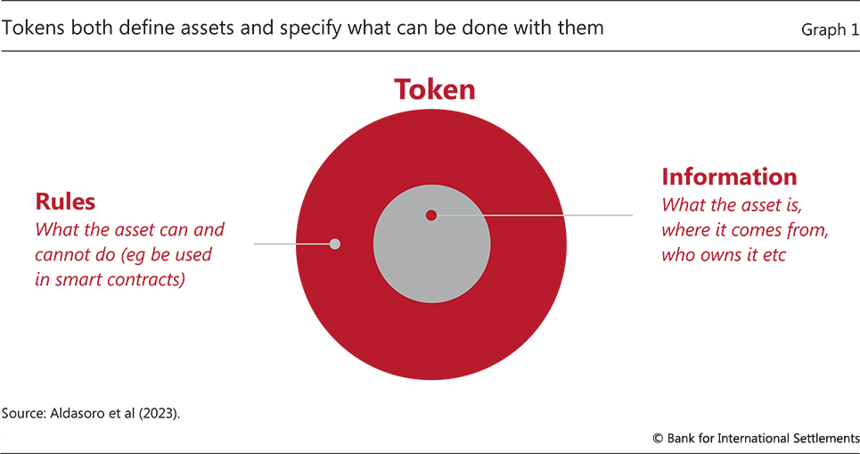
Tokenisation – the process of recording claims on financial or real assets that exist on a traditional ledger on a programmable platform – introduces two important capabilities. First, by dispensing with messaging and the reliance on account managers to update records, it provides greater scope for composability, whereby several actions are bundled into one executable package. Second, it enables the contingent performance of actions through smart contracts, ie logical statements such as “if, then, or else”. By combining composability and contingency, tokenisation makes the conditional performance of actions more readily attainable, even quite complex ones.5
This chapter examines several use cases of such contingent performance of actions. One is in the design of supply chains in which several participants interact under uncertainty and with incentives that may not be perfectly aligned. Another example is the design of banking deposit contracts where built-in contingencies that depend on the actions of other depositors alter the incentives of depositors to be a first mover in a bank run setting. Such contingent deposit contracts could nullify the so-called first-mover advantage.
Many interesting real-world applications require the tokenisation of assets that currently exist in traditional databases. These assets could range from financial securities whose ownership is recorded in securities depositories to real assets, such as commodities or real estate. The tokenisation process for such assets occurs through so-called ramps that define a mapping between assets in traditional databases and their counterparts in tokenised form (Graph 2). The assets in the traditional database are immobilised or “locked” to serve as collateral that backs the tokens issued on the programmable platform. The locking of assets ensures that the transfer of their tokenised counterparts guarantees the transfer of the underlying assets.
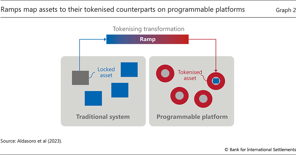
Central bank digital currency and private tokenised monies
The full potential of tokenisation needs a monetary unit of account that denominates transactions, as well as the accompanying means of payment. In crypto, stablecoins that reside on the same platform as other crypto assets perform the role of the means of payment. However, for reasons highlighted already, central bank money and the settlement finality that it brings is a much firmer foundation for tokenisation.6 The full potential of tokenisation is therefore best harnessed by having central bank money reside on the same venue as other tokenised claims. This is because programmable transactions could incorporate settlement using the economy’s unit of account as an essential part of the tokenised arrangement.
For this reason, the development of a wholesale CBDC is core to the functioning of a tokenised environment. As a tokenised means of settlement, wholesale CBDCs would serve a similar role as reserves in the current system, but with the added functionalities enabled by tokenisation. Transactions in wholesale CBDC could incorporate all the features such as the composability and contingent performance of the actions mentioned above. The BIS Innovation Hub, in partnership with central banks around the world, stands at the forefront of experimentation with CBDCs and tokenisation (Box A).
Enhanced digital representations of central bank money could include a retail variant open to use by ordinary users. A retail CBDC is a digital version of physical cash that can be used by households and firms for everyday transactions. By providing the public with a ready way to convert alternative private digital monies into digital cash, ie a direct link to the sovereign unit of account in digital form, the central bank would further support singleness.7
While the role of CBDCs in a tokenised environment is clear, there is greater room for debate concerning the appropriate form of private tokenised money that complements CBDCs. There are currently two main candidates for private tokenised monies: tokenised deposits and asset-backed stablecoins.8 Both represent liabilities of the issuer, who promises customers that they can redeem their claims at par value in the sovereign unit of account. However, tokenised deposits and asset-backed stablecoins differ in how they are transferred and in their role in the financial system. These differences have implications for their attributes as a tokenised form of money that complements CBDCs.
Tokenised deposits could be designed to resemble the workings of regular bank deposits in the current system; see McLaughlin (2021). They could be issued by commercial banks and represent a claim on the issuer. Like regular deposits, they would not be directly transferable. Central banks’ liquidity provision for settlement would continue to ensure smooth functioning of payments.
To bring out the parallels between tokenised deposits and conventional deposits in the current system, consider how a payment is made currently, using deposit balances. When John makes a payment of GBP 100 to Paul, Paul does not receive a GBP 100 deposit at John’s bank. Rather, John’s account balance at his bank is reduced by GBP 100, while Paul’s balance at his bank increases by the same amount. Meanwhile, the adjustments in the individual accounts at the two banks are matched by a transfer in central bank reserves between the two banks. The same payment outcome could be achieved in a tokenised world by reducing John’s tokenised deposit holding at his bank and increasing Paul’s tokenised deposit holding at his, while simultaneously settling the payment through a concurrent transfer of wholesale CBDC (Graph 3). Paul continues to have a claim only on his bank, where he is a verified customer, and has no claim on John’s bank, nor on John.
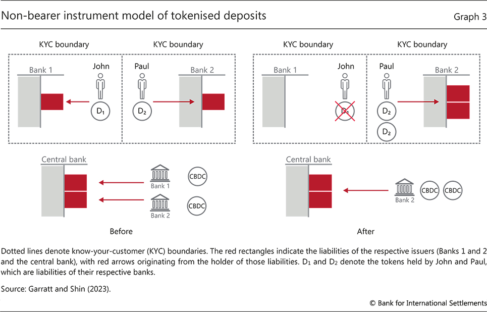
Tokenised deposits would not only preserve but at times enhance some key advantages of the current two-tier monetary system.
First, tokenised deposits would help preserve the singleness of money. In the current system, singleness of money for payments involving commercial bank deposits is achieved because central banks operate settlement infrastructures that guarantee the ultimate transfer of payments at par value in terms of the sovereign unit of account. Tokenised deposits would preserve this arrangement. However, the fact that settlement in wholesale CBDC is automatically triggered through smart contracts would improve the immediacy of the current process, further narrowing time gaps to reduce risks.
Box A
Experiments with wholesale central bank digital currencies and tokenisation
The BIS Innovation Hub stands at the forefront of experimentation with central bank digital currencies (CBDCs) and tokenised assets (Table A1). The work includes projects within and across jurisdictions and in multiple currencies, often in partnership with the private sector.
Experiments with CBDCs have shown that tokenisation can reduce the complexity of securities settlement by facilitating simpler and more direct holding systems, as shown in Project Helvetia. The findings from Helvetia also suggest that using wholesale CBDC, as opposed to linking real-time gross settlement systems to a financial infrastructure, could provide greater scope for future innovation and efficiency gains in the settlement process. In this context, tokenisation facilitates increased automation through the use of smart contracts. It can speed up settlement as tokenised assets typically settle automatically, ie both legs of a transaction settle simultaneously and instantly. Tokenisation also increases operational transparency, as shown in Projects Jura, Dunbar and mBridge. These three completed wholesale CBDC projects focus on use cases where CBDCs were transferred against either another CBDC (payment versus payment, PvP) or tokenised securities (delivery versus payment, DvP). While systems exist to cater to both cross-border PvP and DvP, coverage is not universal in terms of currencies and jurisdictions, and costs are often deemed too high for universal usage. These projects were able to offer new solutions to long-standing operational challenges and policy questions. For example, in Project Jura, subnetworks allow the platform to respect jurisdictional boundaries and data location requirements and notaries allow central banks to control and monitor transactions in their currencies both in terms of payments and PvP settlements. Moreover, programmability allows new types of contingent payment, while certain policy measures (eg capital controls) can be built in from the start.
Beyond CBDCs, other projects have explored the practical and technological complexities of tokenised assets in the context of green finance (Project Genesis) and trade finance (Project Dynamo).
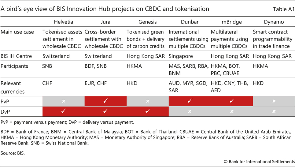
See BIS Innovation Hub (2023).
Second, payments in tokenised deposits settled in wholesale CBDC would ensure finality. By using its own balance sheet as the ultimate means of settlement, the central bank provides the means for ensuring the finality of wholesale payments. As the trusted intermediary, it is the central bank that debits the account of the payer and credits the account of the payee, after which the payment is final and irrevocable. In the above example, finality ensures that Paul does not have a claim on John (or John’s bank), but on his bank only.
Third, tokenised deposits would ensure that banks could continue to offer credit and liquidity in a flexible way. In the current two-tiered monetary system, banks provide individuals and firms with loans and on-demand access to liquidity through, for example, credit lines. Most of the money that circulates in the monetary system today is created in this way. This is in large part possible because the recipients of credit can simultaneously hold deposit accounts at banks, allowing banks to create deposits when making a loan.9 Unlike narrow banking models, this flexibility allows banks to adjust to the needs of firms and households in the light of changing economic or financial conditions. Of course, adequate regulation and supervision are required to prevent excessive credit growth and risk-taking.
Stablecoins are an alternative form of private tokenised money, but they have important shortcomings.10 In contrast to tokenised deposits, stablecoins represent a transferrable claim on the issuer, akin to a digital bearer instrument. A payment using stablecoins transfers the issuer’s liability from one holder to another. Imagine that John holds 1 stablecoin unit (SCU) issued by a stablecoin issuer. When John pays Paul SCU 1, John’s claim on the stablecoin issuer is transferred to Paul, who did not have a claim on that issuer before the transfer. There is no need to update the stablecoin issuer’s balance sheet, and there is no settlement on the central bank’s balance sheet. Whoever holds the instrument has a claim on the issuer and can transfer it without the need for consent or involvement of the issuer. In this case, Paul is left with a claim on an issuer he may not trust.
As stablecoins are tradable, their prices can deviate from par, thus undermining the singleness of money. Deviations from singleness can occur if there are differences in liquidity across stablecoins or if variations in the quality of the backing or characteristics of the issuer lead to differences in the perceived creditworthiness of different issuers. Even higher-order uncertainty can arise, such as that associated with doubts about whether others harbour doubts about the value of a stablecoin, which can lead to discounting and hence undermine singleness.11 For these reasons, as well as the absence of a clear regulatory and supervisory framework and the lack of a central bank as a lender of last resort, there have been multiple recent episodes where stablecoin prices have lost their pegs (Graph 4).
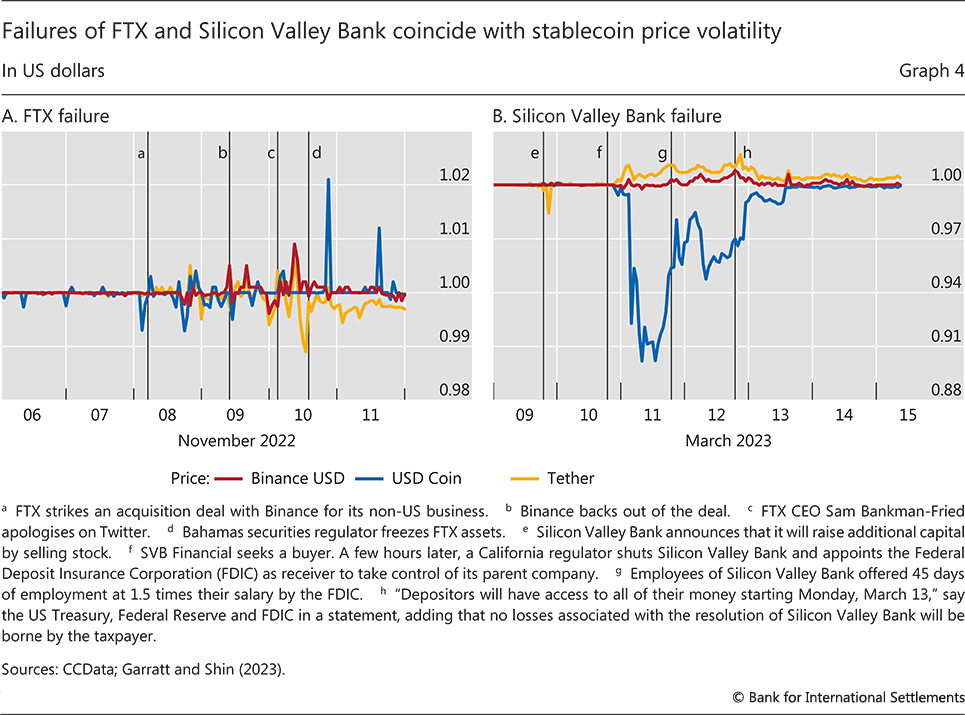
Asset-backed stablecoins also do not allow for the elastic provision of a general means of payment. Any dollar against which a stablecoin is issued should be, at least in principle, invested directly in safe and liquid assets. Stablecoins thus reduce the overall supply of liquid assets that are available for other purposes.12 Even if well regulated and supervised, stablecoin issuers would operate like narrow banks.
Finally, tokenised deposits have advantages over stablecoins in terms of compliance with know-your-customer (KYC), anti-money laundering (AML) and combating the financing of terrorism (CFT) rules. Going back to the example above, Paul holds the liability of the stablecoin issuer after the transfer from John. But the issuer did not perform any identity verification or compliance check on Paul, which creates a risk of fraud. To ensure compliance with KYC, AML and CFT regulation for stablecoins, a significant regulatory overhaul would be necessary.13 In contrast, tokenised deposits, by closely resembling the traditional deposit transfer process, could leverage the existing regulatory and supervisory frameworks for financial institutions.
Achieving seamless interoperability through unified ledgers
The potential of tokenisation lies in its ability to knit together transactions and operations that encompass money and a range of other assets that reside on the programmable platform. Money in tokenised form provides the essential means of payment that mirror the underlying economic transactions. At the heart of the system lies central bank money in tokenised form that facilitates settlement finality.
This section outlines the concept of a unified ledger where central bank digital currencies, private tokenised monies and other tokenised assets coexist on the same programmable platform. In simple terms, a unified ledger could be considered a “common venue” where money and other tokenised objects come together to enable seamless integration of transactions and to open the door to entirely new types of economic arrangement.
The concept of a unified ledger does not mean “one ledger to rule them all” – a sole ledger that overshadows all other systems in the economy. Depending on the needs of each jurisdiction, multiple ledgers, each with a specific use case, could coexist. APIs could connect these ledgers to each other and existing systems (Box B). Over time, they could incorporate new functions or merge as overlaps in scope expand. The scope of a unified ledger would also determine the parties involved in each ledger’s governance arrangements.
Box B
Connecting ledgers through application programming interfaces
A unified ledger combines tokenised money and assets on a common platform. By doing so, it enables programmability, composability and multi-asset atomic settlement. On the road to a unified ledger, an intermediate solution would be to integrate legacy systems and existing infrastructures with new programmable platforms through application programming interfaces (APIs). APIs can interconnect systems and implement ramps that lock assets in traditional ledgers and unlock them in programmable platforms. If well designed, APIs may guarantee settlement finality as conventionally defined (CPSS-IOSCO (2012)). However, because APIs involve multiple systems with different operators and protocols, API implementations cannot achieve atomic settlement. Graph B1 shows three different models that range from the smallest incremental enhancement to a fully fledged unified ledger.
In the first model, an API connects the existing payment system to a programmable platform that contains only a limited number of asset classes (Graph B1.A). The programmable platform does not contain tokenised private monies or central bank digital currency (CBDC). Clearing and settlement of payments are achieved using traditional accounts at banks and via the conventional settlement system (eg a real time gross settlement system). A set of APIs coordinate workflows by sending and receiving messages across systems. The operators from both systems establish the standards for APIs. Settlement finality is achieved in the usual way. However, in this model, atomic settlement involving transactions with private monies, central bank money and other assets would not be feasible.
In the second model (Graph B1.B), the programmable platform contains tokenised private monies and tokenised assets, and APIs connect these to the central bank’s settlement infrastructure. The platform contains no partition for the central bank. Tokenised private money partitions are connected to traditional systems through APIs and smart contracts. These contracts contain rules that ensure that the updating of accounts across participants is accompanied by settlement in central bank money in the traditional settlement system, which is triggered through APIs. This model guarantees atomic settlement for private monies and other assets, but not for transactions that involve CBDC.
In the third model (Graph B1.C), wholesale CBDC, tokenised private monies and tokenised assets coexist on a fully fledged unified ledger. Wholesale CBDCs could be provided in two ways. In the first, CBDCs may take the form of a central bank liability that is issued directly on to the unified ledger. Alternatively, the central bank could tokenise existing reserves using an API that connects the unified ledger to the current reserve system. This system supports settlement finality and atomic settlement for transactions involving wholesale CBDC, private tokenised monies and tokenised assets.
The latter approach is being adopted in the Brazilian Digital Real pilot project (Central Bank of Brazil (2023)).
While the creation of a unified ledger would require the introduction of a new type of financial market infrastructure (FMI), some of the envisaged benefits could also be reaped through more incremental changes to existing systems and interlinking them through APIs into a network of networks. Weighing the pros and cons of a big leap against those of a series of incremental changes is important when considering innovation of any kind but it is especially important for the large discrete changes entailed by new infrastructures such as a unified ledger. Some automated processes for exchanging data that resemble operations in tokenised environments could be achieved by connecting existing systems through APIs. In the short term, modifying existing systems would require lower upfront costs and less coordination among stakeholders than creating a unified ledger.
Yet history shows that incremental fixes have their limits, especially when they accumulate on top of legacy systems. Each new layer would need to look forwards while being constrained by having to look backwards to ensure compatibility with legacy systems. These constraints will become more binding as more layers are added on top, eventually holding back innovative developments. The history of computing and software is replete with such examples.14
For these reasons, it is often the case that harnessing the benefits of technological advances necessitates a fundamental rethink of the financial infrastructure that supports new types of operation. Tokenisation presents another such opportunity, where the introduction of programmable platforms could bring long-term benefits that far outweigh the short-term costs arising from investment as well as the costs and coordination efforts in shifting to new standards and procedures. Of course, the relative balance between the benefits of a unified ledger and those from interlinking existing systems through APIs will depend on the state of technology and the specific needs of each jurisdiction. There is no one size fits all.
The building blocks of a unified ledger
A unified ledger leverages the benefits of tokenisation on a common platform. Based on a secure environment for storing and sharing data through encryption, it could enable new forms of transaction, thus expanding the universe of contracting outcomes.
There are two key aspects to the design of a unified ledger. The first is that it combines all the components needed to complete a transaction on one platform, ie it has everything in one place. The second is that it features money and assets as executable objects, which means they could be transferred safely and securely without going through external authentication and verification processes and without relying on external messaging systems.
The structure of a unified ledger can be described in terms of the following building blocks (Graph 5). The ledger comprises a data environment and an execution environment, which are subject to a common governance framework. The data environment contains the digital representations of money and assets in separate partitions that are owned and operated by the respective competent operating entities (dashed lines). The data environment also includes information necessary for the operation of the ledger, such as the data required for the secure and legal transfer of money and assets. The data environment also encompasses all information necessary to incorporate real-world events into any contingent performance of actions. Information can be a direct result of transactions on the ledger or may be obtained from the outside environment.15
Any operation involving one or more of these elements is carried out in the execution environment, either directly by users or through smart contracts. For each specific application, operations in the execution environment combine only the intermediaries and assets required for each application. For example, a payment between two individuals, executed via a smart contract, would bring together the users’ banks (as providers of tokenised deposits) and the central bank (as provider of CBDC). Should the payment be conditional on some real-world contingency, that information would also be included.
The common governance framework specifies the rules and standards of how the different components interact in the execution environment, as well as which privacy rules apply. Preserving strict confidentiality is a prerequisite if a unified ledger is to be a practical proposition. Confidentiality and data control are achieved in two mutually reinforcing ways: data partitions and data encryption (denoted with a lock in the execution environment). Partitions guarantee that data and information are visible and accessible to only the respective authorised parties for each partitioned domain, ensuring strict confidentiality. At the same time, cryptographic techniques could ensure that data can be shared confidentially as inputs in the execution environment. The details are discussed in the following sections.
Use cases: improving the old
While the monetary system has served society well, its current design could lead to the emergence of pinch points. Digital money currently sits at the edges of communication networks, where it resides in siloed proprietary databases operated by banks and non-banks. External messaging systems are required to link these databases. The separation of messaging, reconciliation and settlement can lead to delays and means that participants often have an incomplete view of completed actions. Consequently, errors may go undetected for longer, leading to higher error resolution costs and increased operational risk. For these reasons, payment processes can be costly, cumbersome, slow and opaque. And they can fall short of meeting users’ changing demands.
The complexity and lack of transparency in existing payment systems is evident even in a simple payment involving customers of two different banks (Box C). A transfer of funds from payer to payee involves a large number of messages, internal checks and adjustments. Participants generally cannot track the progress of their payments in real time. In particular, the payee does not see when the process is initiated, and the payer does not know when it is completed.16
The payment process is even more complex in cross-border transactions, further amplifying frictions. For one, these require international messaging systems on top of domestic ones. Differences in operating hours and/or holidays as well as inconsistencies across operating systems, for example in the form of different messaging standards, can lead to further delays, increasing settlement risk. In addition, the involvement of more intermediaries (eg correspondent banks) increases operational risk. For cross-border payments involving different currencies, there is also foreign exchange (FX) settlement risk, namely the risk that one party to a currency trade fails to deliver the currency owed.17
A unified ledger could improve the way payments are executed. Having private tokenised monies and CBDC on the same platform eliminates the need for the sequential messages across siloed databases. This enables so-called atomic settlement, in which two assets are exchanged simultaneously, such that the transfer of one occurs only upon transfer of the other.18 In the process, settlement, ie the wholesale leg of the payment from one intermediary to another, also occurs instantaneously in wholesale CBDC.19 At the same time, the use of a partitioned data environment with appropriate access controls allows full transparency for the transacting parties, while keeping the transaction private from those who are not involved. Finally, by combining messaging and payment rails on the same platform, the ledger eliminates delays in the payment process, thereby mitigating settlement risk.
Securities settlement could benefit greatly from execution on a unified ledger. The current process for securities settlement involves multiple parties, such as brokers, custodians, central securities depositories, clearing houses and registrars. Accordingly, there is a need for various messaging instructions, money flows and reconciliation procedures, all of which lengthen the process, increase the costs and expose parties to additional risks. By bringing tokenised money and securities together on a programmable platform, some of these risks could be mitigated by shortening settlement lags and obviating the need for messaging and reconciliation. Moreover, the simultaneous execution of the delivery and payment legs could expand the scope of securities covered in delivery-versus-payment (DvP) arrangements, further contributing to risk mitigation. Box D discusses this possibility in more detail.
Box C
Messaging in a standard person-to-person wire transfer
Messaging that governs digital money is currently located at the edges of communication networks and money transfers involve multiple messages through third-party messaging systems. At each step of the process, participants often have only a limited view of the completed actions.
The complexity and lack of transparency in existing payment systems can be illustrated with a simple example of a wire transfer from Alice to Bob (Graph C1). The process begins with Alice sending a payment request to her bank using the bank’s mobile app (step 1). Bank A responds by debiting Alice’s account by the transfer amount together with any fees (step 2) and sending a payment order to the settlement system (step 3). The settlement system debits Bank A’s settlement account and credits Bank B’s account (step 4) and sends an advice of credit with a reference number to Bank B (step 5). There follows an acknowledgement with a reference number to Bank A (step 6). Bank B must ensure Bob has an account and perform any know-your-customer or anti-money laundering checks (step 7). If any of these checks fail, then Bank B will need to send a reversal request to the settlement institution (potential step 8a shown in light grey). Otherwise, Bank B credits Bob’s account (step 8b) and sends a message to Bob notifying him of the adjustment to his account (step 9).
In some payment systems Bank B must accept the transfer by Bank A before it takes place. In this case, steps 5 and 7 come before step 4. It is also worth emphasising that in the description provided in Graph C1, Alice is not notified that Bob has received the transfer. This can be achieved through additional messages from Bank B to the settlement system (step 10), from the settlement system to Bank A (step 11), and then with a final confirmation message from Bank A to Alice (step 12). These steps appear in light grey in Graph C1 to show that they are not common to all systems.
Another important use case is the mitigation of settlement risk in the multi-trillion dollar FX market. Existing netting and payment-versus-payment (PvP) mechanisms help to mitigate settlement risk, but do not fully eliminate it, not least as existing PvP arrangements are at times unavailable, unsuitable for some trades or deemed too costly by market participants.20 Atomic settlement around the clock, instead, could eliminate settlement lags. Moreover, smart contracts that combine currencies with authorised FX providers could allow more currencies to be integrated on a common platform at a lower cost, expanding the scope of PvP arrangements.
Box D
Streamlining securities settlement through a unified ledger
Today, the process of trading securities and settling securities transactions involves multiple parties, with a myriad of messaging instructions, reconciliation efforts and money flows involved (Graph D1). Central securities depositories (CSDs) electronically manage securities either directly or indirectly (eg through a custodian) for the security’s beneficial owner. A securities buyer or seller initiates the process by instructing her broker or custodian to initiate the trade. During the time between trading and final settlement (the “settlement cycle”, which can take up to two days), parties are exposed to replacement cost risk (ie the risk of a trade failing to settle and having to be replaced at an unfavourable price). In addition, during the settlement process itself, counterparties are exposed to principal risk (ie the risk that one counterparty does not fulfil the agreement – failing either to pay or to deliver the security). The CSD must verify the identity of account holders and ensures reconciliation and confirmation of what is being settled with the relevant third parties (eg clearing agents).
A unified ledger could reduce these risks by reducing the number of counterparties and shortening confirmation and reconciliation times. If both tokenised money and securities are hosted on a common platform, the risks and costs that arise from having them reside in separate ledgers can be reduced substantially. The simultaneous execution of the delivery and payment legs could also expand the scope of securities covered in delivery-versus-payment (DvP) arrangements, helping to mitigate principal risk between counterparties. Appropriate liquidity saving mechanisms would need to be instituted, as atomic settlement also puts higher liquidity demands on the system – much like the move from deferred net settlement to real-time gross settlement.
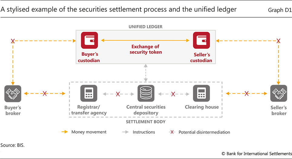
Use cases: enabling the new
Beyond improving existing processes, a unified ledger could open the door to entirely new types of “arrangements and transactions” that expand the universe of possible contracting outcomes. This is made possible through the combination of smart contracts, a secure and confidential environment for storing and sharing information and the execution of transactions enabled by tokenisation.
Smart contracts increase the scope for successful coordination. In many instances, mutually beneficial outcomes cannot be achieved when participants need to undertake costly joint efforts. The reason is that individual participants may have an incentive to free ride on the contribution of others. Contingent performance promises to overcome such coordination problems. For example, a smart contract could specify that each participant contributes only a certain amount to a joint venture if all other participants also contribute. This way, free-riding is eliminated.
Overcoming coordination problems may be particularly useful in the context of banking, where the use of contingency in term deposit contracts could contribute to the stability of bank funding and the banking sector more generally. Typically, term deposit contracts are bilateral arrangements between the bank and the depositor. Yet from time to time, the value of deposits can depend on the collective decisions of all depositors, especially during stress periods in the banking sector. In this context, strategic uncertainty arises as early withdrawals are met on a first-come, first-served basis, while the bank invests funds in illiquid assets. Depositors who withdraw first thus have an advantage and this can lead to bank runs. This problem could be mitigated by allowing explicit coordination through the design of new types of deposit contracts that impose contingent performance of actions on depositors. Such contracts could ensure that early withdrawers do no better than late withdrawers, thus eliminating the motivation to withdraw funds purely out of fear that others might do the same. This type of arrangement would not prevent all potential types of run from occurring, but it could mitigate the textbook case of first-mover advantage and coordination failures.
Supply chains are another possible use case that would make full use of a unified ledger’s capabilities to incorporate real-time information into smart contracts. The problem of supply chain financing has been a notoriously difficult one to solve in real-world settings. Supply chain financing has attributes of a DvP problem as explained below, but one which also features uncertainty and information asymmetries about the underlying state of the world.
Graph 6 depicts a stylised supply chain. A buyer (usually a large firm) purchases goods from suppliers (often small and medium-sized enterprises, SMEs), which in turn require goods from other suppliers for production. A common problem is that the buyer would prefer to pay for the goods only once delivered. However, suppliers need to pay their workers and purchase materials to produce the goods beforehand. They thus require some form of financing until they receive payment from the buyer. For well known reasons, including the risk that the buyer will not pay upon delivery, obtaining trade credit usually requires firms to pledge collateral.21
For example, an SME in Italy might expect delivery of intermediate goods via ship from its Indian supplier in one month’s time. To set up production now, it can pledge these goods as collateral to obtain a loan from a bank or its suppliers. Should the company default, the creditor can reclaim the collateral. However, creditors might be reluctant to provide sufficient credit or charge a prohibitively high interest rate, as the collateral might lose value due to pirate attacks or storm damage to the ship. The firm might also engage in fraudulent behaviour and try to pledge the collateral to different parties simultaneously, which is common in trade finance.22 These frictions to obtaining financing imply that suppliers often have to rely on their own funds to meet their working capital needs.
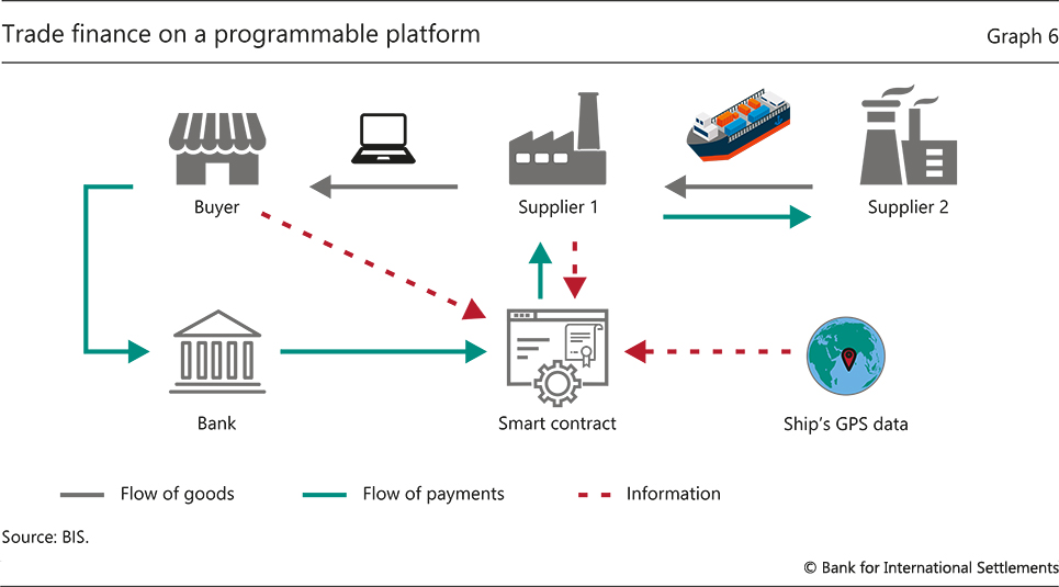
By combining the different components of the supply chain relationships and the steps of the financing process in one place, a unified ledger could mitigate the problems plaguing trade finance. Contracts that formalise the conditional performance of actions could eliminate incentive problems. Smart contracts could specify an automatic payment from the buyer to its suppliers upon delivery of goods, or partial early payment when intermediate steps are reached. This way, creditors would not need to worry about the risk that the buyer will not honour its obligations. Banks could extend loans featuring smart contracts that act upon real-time information on shipments provided by internet-of-things (IoT) devices, such as GPS data. In the above example, the interest rate could automatically fall, or additional credit be granted, once the ship passed the Horn of Africa, a notoriously high-risk area for piracy. This way, suppliers could finance part of their working capital needs as early as the production phase. Finally, because all trade finance contracts would be written on a shared ledger, it would be impossible to write duplicate loan contracts tied to the same collateral, which would further enhance lenders’ willingness to extend credit to firms.
Tokenisation can help solve many of the issues plaguing international trade among small firms.
In addition, by providing a secure and confidential environment for storing and sharing information, the ledger could harness the benefits of data to lower the cost of and improve access to credit. The use of data can bring both benefits and costs. Data allow lenders to better assess the riskiness of borrowers, reducing both costs and the need for collateral. For example, lending by big techs, which use big data and machine learning to assess credit risk, is less sensitive to changes in real estate collateral values than bank credit (Graph 7.A).23 But network effects can lead to market concentration and ultimately higher costs for households and firms: the analysis of large troves of data enhances existing services and attracts further users, which in turn create new data, leading to a data-network-activities or “DNA” loop.24 Moreover, privacy concerns can make individuals reluctant to share their data. With data-sharing technologies (discussed below), mathematical computations can be performed directly on encrypted or anonymised data. Users hence retain control over their data when sharing them on the ledger. Through improved data-sharing arrangements, the unified ledger could enhance financial inclusion, in particular among disadvantaged segments of the population such as racial minorities and low-income households. These “thin credit file” applicants stand to benefit disproportionately from screening via non-traditional data: as banks’ traditional credit scores are noisier indicators of their default risk than for other groups of the population, additional data yield a more precise signal of their credit quality (Graph 7.B).25 In turn, lenders can offer loans at lower rates.
Through encryption technology, a unified ledger could also enable new ways to enforce AML and CFT requirements. Financial institutions safeguard highly sensitive and proprietary data that often need to be kept confidential by law. However, the inability to share such sensitive data without exposing confidential information can hinder efforts to combat money laundering and other illicit activities. The use of a unified ledger could provide transparent and auditable records of transactions, transfers and ownership changes. Encryption methods allow financial institutions to share these data confidentially with each other and across borders to detect fraud and money laundering while remaining compliant with domestic data regulations.
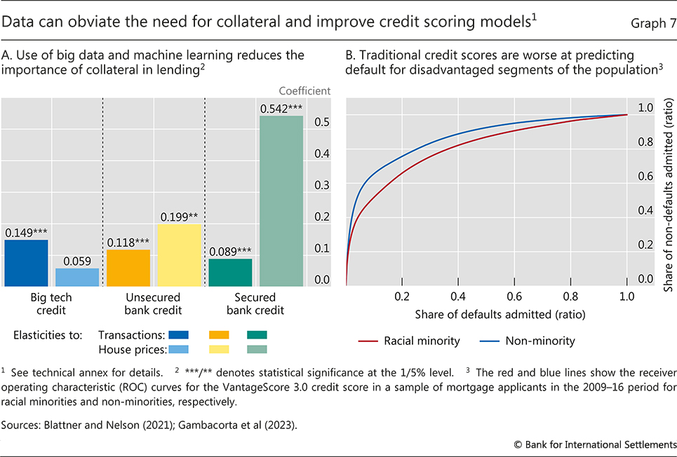
These benefits could be further enhanced by leveraging tokenisation and the dual nature of tokens encompassing both identifying information and the rules governing transfer. In the case of payments, for example, supervisory compliance requirements that depend, among other things, on the transacting parties, their location and the type of transfer could be directly embedded into the token.26 While not undertaken in the context of a unified ledger, the BIS Innovation Hub’s Project Aurora is exploring how privacy-enhancing technologies and advanced analytics might be leveraged to combat money laundering across financial institutions and borders.
The combination of smart contracts, information and tokenisation could also improve the issuance of and investment in securitised assets and bonds. One example is mortgage-backed securities (MBS), which pool mortgage loans into tranches of debt that are subsequently purchased by investors. Yet even in the deeply liquid $12 trillion US MBS market, the process of securitisation involves over a dozen intermediaries.27 Automation through smart contracts could eliminate time lags in information and payment flows, streamlining the securitisation process. A token could integrate real-time data on borrower repayments and how they are pooled and distributed to investors, further reducing the need for intermediaries.
Another use case is in green finance. The BIS Innovation Hub’s Project Genesis illustrates some of the benefits of tokenisation and smart contracts. The project involves a platform from which an investor can download an app and invest any amount into tokenised government bonds that fund a green investment. Over the bond’s life cycle, smart contracts allow the investor not only to see accrued interest, but also to track in real time how much clean energy is being generated and how far carbon emissions are being reduced as a result of the investment. Moreover, the investor can sell the bond in a transparent secondary market.
Taken together, these examples show how applications of the unified ledger have the potential to enhance the current monetary and financial system. For existing processes, a unified ledger could seamlessly automate and integrate transactions. And by leveraging the benefits of tokenisation and providing a secure environment for sharing data, a unified ledger could enable altogether new types of transaction.
Guiding principles for a unified ledger
Any application of the unified ledger concept should adhere to a number of high-level guiding principles. First and foremost, any application should be fully integrated with the two-tiered structure of the monetary system. In this way, the central bank could continue to support the singleness of money by providing settlement in wholesale CBDC, and the private sector could continue to innovate to the benefit of households and firms. In addition, there are important principles related to its scope and governance. These will specify how best to ensure a level playing field and foster competition, as well as how to ensure data privacy and operational resilience. The concrete implementation of these principles ultimately depends on the needs and preferences of each jurisdiction as well as the details of the specific application.
Scope, governance and competition
The first important question regards the scope of the ledger. As discussed above, the concept of a unified ledger does not exclude a multiplicity of coexisting ledgers, each with a specific use case. In practice, the concept is likely to be applied first to specific applications where benefits are more immediate (Box E). For example, one ledger could aim at improving securities settlement, involving only the relevant parties, while another could pertain to trade finance in, say, the shipping industry. Starting from specific use cases, the ledger’s scope could expand over time as it includes additional assets and entities. Ultimately, the scope of the ledger will depend on the specific needs and constraints of each jurisdiction.
Irrespective of its scope, a unified ledger would effectively be a new type of FMI or a combination of multiple FMIs. As such, a natural starting point for drawing up standards would be the Principles for financial market infrastructures28 which, in addition to setting out requirements for access, safety and operational resilience, state that FMIs should provide clear and certain final settlement (Principle 8) in central bank money where practical and available (Principle 9). These principles apply to a wide range of infrastructures such as payments systems, central securities depositories, securities settlement systems, central counterparties and trade repositories.
The scope of the ledger has direct implications for its governance arrangements, competitive design and the incentives to participate.
Governance of a unified ledger could follow existing arrangements, whereby central banks and regulated private participants take part in governance under established rules. For example, when money and payments are involved on a ledger, the central bank will necessarily play a role as the provider of the ultimate settlement asset. Its specific involvement in governance arrangements could take various forms, much as it does in the case of traditional payment systems, where public ownership, regulation and oversight, as well as private mutual ownership are all viable options.29 To ensure integrity, regulated and supervised private participants should remain in charge of customer-facing activities. They should also adhere to established KYC, AML and CFT regulations, as well as perform ongoing due diligence to ensure compliance with privacy regulations.
Box E
The tokenisation continuum
Tokenisation – the process of recording claims on real or financial assets that exist on a traditional ledger on a programmable platform – needs to overcome several economic, legal and technical challenges.
An intrinsic feature of many markets is economic friction generated by uncertainty and misaligned incentives, which can be mitigated by trusted intermediaries. For example, when a bank makes a loan to a non-financial firm, the borrower knows more about the quality of its project and the effort devoted to it. To ensure that funds are put to their intended use, lenders need to screen the quality of the borrower ex ante and monitor performance ex post. Technology alone is unlikely to overcome these market imperfections, leaving a role for intermediaries to screen borrowers.
Tokenisation efforts must also address legal issues. Rules and regulations governing tokenised assets must be aligned with those of their non-tokenised counterparts, which requires regulatory coordination to prevent unintended consequences such as shadow activities, theft and regulatory arbitrage. This task is easier for assets subject to legal frameworks and regulations that are standardised and can be easily translated into a computer algorithm. Broader issues include those pertaining to investor and consumer protection, cyber security and regulatory compliance across borders.
There are also technical challenges, especially in the design of ramps that map assets on traditional ledger systems to their tokenised counterparts. Ramps lock assets in their platform of origin as collateral for the tokens that are issued on the programmable platform. Locking and unlocking the original assets requires seamless interaction and coordination across systems. For example, to lock a property on a platform, the on-ramp would need to ensure that the property is no longer tradable outside the platform. As property titles are kept in disparate local registries, full automation could be difficult without the involvement of (offline) intermediaries. Generally, the feasibility of on-ramping and the associated benefits on the programmable platform will depend on the level of automation and harmonisation of the systems of origin.
As discussed in a recent BIS study, these aspects define a tokenisation continuum (Graph E1). It highlights a trade-off: for those applications where tokenisation is easiest, per-unit gains are likely to be modest; but the gains are likely to be largest for applications where tokenisation is most difficult. Therefore, in the short term, tokenisation could focus on identifying assets that are suitable for tokenisation and traded in large volumes.
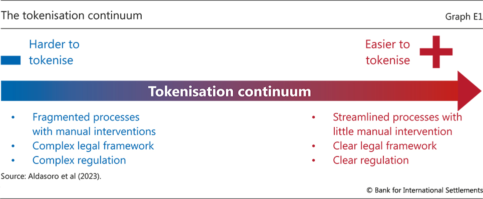
See Aldasoro et al (2023).
The demands on governance arrangements increase with the scope of the ledger. For example, a unified ledger for cross-border payments would require seamless interoperability across private payment service providers (PSPs) and central banks located in various jurisdictions with different regulatory and supervisory frameworks. It would hence require significant harmonisation efforts across jurisdictions. A ledger that targets domestic securities settlement, on the other hand, would require less intensive coordination efforts.
An open and level playing field is important for competition and financial inclusion. From a public policy perspective, it is critical to consider how the introduction of a common platform may affect the industrial organisation of money and payments, and ultimately of the entire financial system. Promoting healthy competition between private actors through open platforms can foster innovation and lower costs for end users by reducing rents. By designing platforms and attendant regulations with these goals in mind, public authorities can help ensure that network effects work for the benefit of consumers. To this end, the use of encryption techniques such as homomorphic encryption could help prevent the concentration of data within centralised entities, and hence the emergence of dominant players.
An important challenge in promoting competition is providing the right economic incentives for potential participants. Without the right incentives, PSPs might decide not to join. Efforts to centralise over-the-counter (OTC) bond markets offer valuable lessons.30 Trading government bonds on an exchange, as opposed to over the counter, can lead to lower costs through improved matching and greater liquidity, especially during stress periods.31 However, high entry and operating costs or benefits from established investor-dealer relationships can deter some players from joining. As the main players in OTC markets, dealers also often enjoy market power and high profits, which can make them reluctant to join a common platform.32 But unless a sufficient number of players join, there may be insufficient liquidity and virtuous network effects cannot take hold. The experience from the introduction of fast payment systems suggests that mandating participation while simultaneously providing an infrastructure that allows for private sector innovation can be key to ensuring adoption.33 Once the benefits of network effects unfold, new players will join voluntarily.34
Data privacy and operational resilience
By bringing together money, assets and information on a common platform, a unified ledger raises important issues about data privacy and operational resilience.
Adequate safeguards are necessary to protect users’ privacy. The concentration of different types of data, possibly including transaction data in combination with information on geolocation and purchased products or services, raises concerns about data theft and abuse.35 As a fundamental right, privacy requires a conservative approach to data management on the unified ledger. Commercial secrecy is no less important. Businesses may be hesitant to participate in a unified ledger application unless they can protect confidential information such as smart contract code and transaction logs.
A key element to guaranteeing privacy is to create partitions in the ledger’s data environment (Graph 5). Each entity, such as banks or the owners of tokenised assets, will see only transactions and associated data on their own partition. Updates to the data environment are initiated by the account owners through use of their private keys. These private keys are used to authenticate and authorise transactions, ensuring that only legitimate account owners can make changes to their own partition of the ledger’s data environment.
In addition, encryption and other privacy-preserving technologies can ensure the safe sharing and use of data. When different entities interact in a transaction, information from different partitions needs to be shared and analysed in the execution environment. Secure data-sharing technologies enable mathematical computations to be performed directly on encrypted or anonymised data, without revealing sensitive information. Some intermediaries and users may be more willing to share data in encrypted form with other parties, which could foster competition and innovation rather than market concentration and captive behaviour. Commercial secrecy can be maintained by encrypting individual smart contracts. Only the code owner, or parties designated by the code owner, would have access to the contract details.
Various privacy-preserving technologies can protect confidential and personal data in a unified ledger, each with its own benefits and costs, depending on the specific application. Table 1 summarises the key characteristics of selected technologies and the trade-offs involved in their use. Homomorphic encryption and differential privacy allow users to share their data with other parties in encrypted form. Secure multi-party computation and federated learning, on the other hand, enable entities to use common machine learning algorithms while keeping their data in their local partitions. These methods differ in terms of their degree of privacy protection, computational burden and ease of implementation.36
A concrete example of how encryption technology might be used is a small bank that would like to apply a big tech’s advanced machine learning model to assessing the credit risk of its loan applicants. Traditionally, the bank would have to grant the larger player access to its data for this task, which requires a great level of trust that the data will not be used to competitively undermine the small bank. With homomorphic encryption or similar methods, however, the bank can send encrypted data and take advantage of the big tech’s analytic services without handing over the actual data. The big tech, in turn, could further improve its algorithms as they are trained on larger data sets.
As institutions that serve the public interest with no commercial interest in personal data, central banks could play a crucial role in designing ledger applications where privacy safeguards are implemented from the ground up. The ledger could be designed to embed privacy laws directly into the programming of tokens. In many cases, data privacy laws give consumers the opportunity to grant or deny third parties consent to use their data. For example, the European Union’s General Data Protection Regulation gives its citizens the “right to be forgotten” by asking firms to delete their personal data. Likewise, the California Consumer Privacy Act endows Californians with the right to know what personal information is being collected and to prevent its sale or ask for its deletion. However, it is often difficult for users to exercise their options effectively, and to verify whether firms have actually deleted their data. By embedding the option to prevent the sale of data or to delete them directly into a smart contract specific to a certain token and transaction (eg payment data should only be accessible by certain institutions), data privacy laws could be made more effective.
Beyond privacy protection, rising costs from cyber attacks (Graph 8.A) highlight the need for strong institutional and legal safeguards for cyber resilience. Safeguarding the integrity and confidentiality of the ledger’s data requires multiple layers of security such as encryption, authentication, access controls, monitoring and regular security audits. A cyber attack on a critical FMI or ledger could not only entail significant monetary and reputational damage, but also lead to widespread disruption in the financial system and ultimately inflict significant societal costs.37 The more comprehensive the ledger, the bigger the risks of a single point of failure and therefore the larger the potential associated costs. An appropriate level of investment in cyber resilience and security is therefore paramount.
A unified ledger could help ensure a sufficient level of investment in cyber security. Cyber security is a public good. If one institution spends more to protect its own infrastructure, it makes the system as a whole safer, thereby benefiting all other institutions. However, given such positive externalities, the classical problem of under-investment by private parties arises.38 Collectively, financial institutions will spend too little on cyber security (Graph 8.B). The unified ledger, sustained by a public-private partnership that internalises these externalities, could overcome this issue. It would lead to greater investment in cyber security, increasing overall system resiliency.
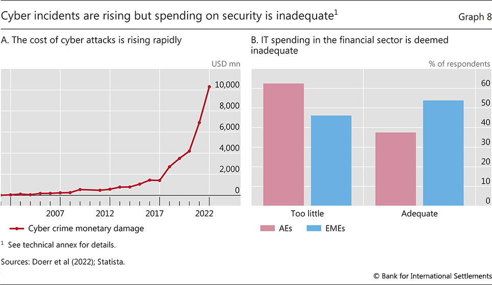
Conclusion
To realise the full benefits of innovation in money, payments and a broader range of financial services, it is crucial to have a vision for the future monetary system and for the role of central banks in driving innovation to meet evolving needs. Given the unpredictable nature of innovation, the focus should be on building a monetary system that is adaptable enough to support safe and sound innovation by the private sector, in any form that this may take.
This chapter has presented a blueprint for a future monetary system that harnesses the transformative potential of tokenisation to improve existing structures and open up new possibilities. This blueprint has sketched out a new financial market infrastructure – a unified ledger – that integrates CBDCs, tokenised deposits and other tokenised claims on financial and real assets in one place.
A unified ledger has two key advantages. First, it provides a venue where a broader array of contingent actions and financial transactions could be seamlessly integrated and automatically executed. In this way, it enables simultaneous and instantaneous settlement. In contrast to the crypto world, settlement in central bank money ensures the singleness of money and the finality of payments. Second, by having everything in one place, it allows new types of contingent contracts that serve the public interest by overcoming obstacles associated with information and incentive problems.
The ideas behind the unified ledger show how the future monetary system might evolve. In practice, the specific needs and constraints of each jurisdiction will dictate which applications of the concept will take root first, and on what scale. Along this journey, multiple ledgers, each catering to specific use cases, could coexist and interconnect through APIs to ensure interoperability.
Crucially, this journey requires a shift in emphasis from individual experimentation to joint innovation. Public-private collaboration is essential to develop technological solutions, establish common platforms and ensure proper oversight and supervision. Through cooperation, innovation and integration, it is possible to pave the way for a monetary system that builds on trust, enables new economic arrangements, enhances the efficiency and accessibility of financial transactions and responds to the evolving demands of households and firms.
Endnotes
1 Schnabel and Shin (2004) provide a historical account of bills of exchange, their evolution from instruments in the payment system to sophisticated instruments of credit, and their role in fostering the growth of trade and commerce. Related discussions are also presented in Quinn and Roberds (2015, 2016) and Frost et al (2020), who also discuss how the Bank of Amsterdam took on a lender of last resort function in the 1763 panic, providing emergency liquidity by accepting a broader range of collateral, and with open market operations.
2 For further elaboration on the structural flaws of crypto see BIS (2022) and Boissay et al (2022).
3 See Carstens (2023b).
4 See Carstens (2023a).
5 Token-specific contracts also allow for the ability to transfer fractions of a token, so-called fractionalisation. Fractionalisation could lower the barriers to entry for households, thus helping to widen financial inclusion.
6 See BIS (2022).
7 See Cunliffe (2023).
8 Asset-backed stablecoins are by far the most prevalent form of stablecoin. They are usually pegged to a numeraire, such as the US dollar, and backed by assets such as government bonds, short-term corporate debt or bank deposits. The issuer typically manages the underlying collateral and coordinates the coins’ redemption and creation. Currently, stablecoins are used mainly within the crypto system and are typically provided by unregulated issuers.
9 See McLeay et al (2014).
10 This discussion is based on stablecoins of the safest possible variety, namely those fully backed by the safest and most liquid assets. Other varieties such as those backed by risky assets or algorithmic stablecoins do not represent a viable alternative (BIS (2022)).
11 See Garratt and Shin (2023).
12 See Garratt et al (2022).
13 These considerations would also be relevant to retail CBDC. However, similar measures that apply to cash today, such as the Financial Action Task Force requirements, could apply to retail CBDC.
14 For example, Lotus 1-2-3 was the standard spreadsheet program throughout the 1980s and into the early 1990s. It was widely used by financial traders, portfolio managers and analysts in investment and commercial banks, brokerage houses and money management companies. Despite various updates, technical setbacks meant that Lotus was struggling to keep pace with the rapid advances in computing power. In the early 1990s, Lotus was surpassed by Microsoft’s Excel, which provided new functionalities and easier usability through a graphical user interface. Similarly, a key reason why smartphones replaced earlier versions of the cell phone was not because they were better for making calls or sending texts, but because they let third parties use their creativity in developing new products and services through apps.
15 Real-world information can be represented on the ledger in two ways. First, via oracles, which are third parties that enter data onto the unified ledger so that they can be directly referenced by smart contracts. Second, via application programming interfaces (APIs). The so-called oracle problem (Duley et al (2023)), which hinders the use of real-world data on decentralised platforms, would not apply, as the unified ledger would use a trusted and mutually accepted set of rules and procedures for data access and conflict resolution in the event of discrepancies.
16 In the case of a card payment from a customer to a merchant there is an additional authentication and verification process that involves the merchant, the purchaser’s bank, the acquiring bank and, in many cases, an access control service that verifies the payment instrument (eg debit/credit card).
17 See CPMI (2023).
18 Atomic settlement involves the reduction of settlement lags (potentially to zero, ie “instant settlement”), while extending the functionality of delivery-versus-payment (DvP) and payment-versus-payment (PvP) arrangements such that multiple linked transactions by various parties can be bundled and settled together (“simultaneous settlement”). See Bech et al (2020) and Lee et al (2022).
19 Another improvement from the adoption of a unified ledger relates to the transaction initiation process. Most person-to-business transactions currently involve an initial validation/verification process that involves contacting an intermediary, verifying the customer’s identity and the payment instrument (eg the debit card using the CVV code) and having all these checks communicated to all relevant participants (eg the buyer, the merchant, the buyer’s bank and the acquiring bank). On a unified ledger, these steps are replaced by the use of private and public keys, which confirm legitimate ownership of funds.
20 More broadly, PvP arrangements may add to funding liquidity risks, as funding is needed to carry out a transaction when required.
21 See Costello (2019). Project Dynamo by the BIS Innovation Hub also investigates how tokenisation could improve supply chain finance.
22 See Association of Certified Fraud Examiners (2022).
23 See Gambacorta et al (2023).
24 These problems became particularly acute with the entry of large technology firms into financial services. See Boissay et al (2021).
25 See Blattner and Nelson (2021) and Doerr et al (2023).
26 See Auer (2022).
27 For example, the so-called servicer collects borrower repayments, pools them and forwards them to a trustee. The trustee then distributes the pooled repayment to security holders according to the structure set in the transaction documents.
28 See CPSS-IOSCO (2012).
29 See Manning et al (2009).
30 Most OTC markets rely on large financial institutions (dealers) to intermediate between investors.
31 Kutai et al (2023) argue that two main reasons can explain this: the possibility of conducting all-to-all trading, and the ability to generate efficiency gains from instant netting of bilateral settlement obligations.
32 See Allen and Wittwer (2023).
33 See Duarte et al (2022).
34 Evidence from the mandate to trade index credit default swaps in swap execution facilities suggests as much; see Riggs et al (2020).
35 See Armantier et al (2021) and Chen et al (2023).
36 Privacy-preserving technologies are based on various methodologies. HE uses the principle of additive and multiplicative homomorphism to enable computations on encrypted data, yielding the same result as if the computations were performed on the original data. SMPC allows multiple parties to jointly compute a function without revealing their input values. However, as the number of parties increases, SMPC may entail higher communication costs. FL allows each party to train a machine learning model separately without sharing their data. Instead, parties only reveal their updated model parameters to a third or central party to collectively build a better machine learning model by aggregating the parameters. DP adds calibrated noise to the original data to protect the privacy of the data. However, there is a trade-off between accuracy and privacy in DP, as improper calibration of noise can result in inaccurate results.
37 See Eisenbach et al (2022).
38 See Anand et al (2022), Doerr et al (2022) and Garratt and Schilling (2022).
Technical annex
Graph 7.A: Each bar reflects the coefficient estimate of the elasticity of credit to changes in firms’ transaction volume or local house prices in firm-quarter regressions.
Graph 7.B: ROC curves plot the fraction of non-defaults admitted for a given score cutoff against the fraction of defaults admitted.
Graph 8.A: Based on cyber crimes reported to the Internet Crime Complaint Center (IC3) of the Federal Bureau of Investigation (FBI).
Graph 8.B: Share of respondents who selected each respective answer to the question “Do you think that investment on cyber security has been too little/adequate/too much over the past year?”.
References
Aldasoro, I, S Doerr, L Gambacorta, R Garratt and P Koo Wilkens (2023): “The tokenisation continuum“, BIS Bulletin, no 72, April.
Allen, J and M Wittwer (2023): “Centralizing over-the-counter markets?”, Journal of Political Economy, forthcoming.
Anand, K, C Duley and P Gai (2022): “Cybersecurity and financial stability”, Deutsche Bundesbank Discussion Papers, no 08.
Armantier, O, S Doerr, J Frost, A Fuster and K Shue (2021): “Whom do consumers trust with their data? US survey evidence“, BIS Bulletin, no 42, May.
Association of Certified Fraud Examiners (2022): “Occupational fraud 2022: a report to the nations”.
Auer, R (2022): “Embedded supervision: How to build regulation into decentralized finance”, Cryptoeconomic Systems, vol 2, issue 1.
Bank for International Settlements (BIS) (2022): “The future monetary system“, Annual Economic Report 2022, June, Chapter III.
Bank for International Settlements Innovation Hub (BISIH) (2023): “Lessons learnt on CBDCs”, report to the G20, forthcoming.
Bech, M, J Hancock, T Rice and A Wadsworth (2020): “On the future of securities settlement“, BIS Quarterly Review, March, pp 67–83.
BIS Committee on Payments and Market Infrastructures (CPMI) (2023): “Facilitating increased adoption of payment versus payment (PvP) – Final report“, March.
Blattner, L and S Nelson (2021): “How costly is noise? Data and disparities in consumer credit”, working paper.
Boissay, F, T Ehlers, L Gambacorta and H S Shin (2021): “Big techs in finance: on the new nexus between data privacy and competition“, BIS Working Papers, no 970.
Boissay, F, G Cornelli, S Doerr and J Frost (2022): “Blockchain scalability and the fragmentation of crypto“, BIS Bulletin, no 56, June.
Carstens, A (2023a): “Innovation and the future of the monetary system“, keynote speech at the Monetary Authority of Singapore, 22 February.
— (2023b): “The value of trust“, speech at award ceremony, King of Spain Prize in Economics, Madrid, 6 March.
Central Bank of Brazil (2023): “Motivations for the Brazilian Digital Real pilot”, Voto 31/2023, 14 February.
Chen, S, S Doerr, J Frost, L Gambacorta and H S Shin (2023): “The fintech gender gap”, Journal of Financial Intermediation, vol 54.
Committee on Payment and Settlement Systems and Technical Committee of the International Organization of Securities Commissions (CPSS-IOSCO) (2012): Principles for financial market infrastructures, April.
Costello, A (2019): “The value of collateral in trade finance”, Journal of Financial Economics, vol 134, no 1, pp 70–90.
Cunliffe, J (2023): “The shape of things to come: innovation in payments and money”, speech at the Innovate Finance Global Summit, London, 17 April.
Doerr, S, L Gambacorta, T Leach, B Legros and D Whyte (2022): “Cyber risk in central banking“, BIS Working Papers, no 1039.
Doerr, S, L Gambacorta, L Guiso and M Sanchez del Villar (2023): “Privacy regulation and fintech lending“, BIS Working Papers, no 1103.
Duarte, A, J Frost, L Gambacorta, P Koo Wilkens and H S Shin (2022): “Central banks, the monetary system and public payment infrastructures: lessons from Brazil’s Pix“, BIS Bulletin, no 52, March.
Duley, C, L Gambacorta, R Garratt and P Koo Wilkens (2023): “The oracle problem and the future of DeFi”, BIS Bulletin, forthcoming.
Eisenbach, T, A Kovner and M Lee (2022): “Cyber risk and the US financial system: A pre-mortem analysis”, Journal of Financial Economics, vol 145, no 3, pp 802–26.
Frost, J, H S Shin and P Wierts (2020): “An early stablecoin? The Bank of Amsterdam and the governance of money“, BIS Working Papers, no 902.
Gambacorta, L, Y Huang, Z Li, H Qiu and S Chen (2023): “Data vs collateral”, Review of Finance, vol 27, no 2, pp 369–98.
Garratt, R and L Schilling (2022): “Optimal data security with redundancies”, working paper.
Garratt, R, M Lee, A Martin and J Torregrossa (2022): “The future of payments is not stablecoins”, Federal Reserve Bank of New York, Liberty Street Economics, February.
Garratt, R and H S Shin (2023): “Stablecoins versus tokenised deposits: implications for the singleness of money“, BIS Bulletin, no 73, April.
Kutai, A, D Nathan and M Wittwer (2023): “Exchanges for government bonds? Evidence during COVID-19”, mimeo.
Lee, M, A Martin and B Müller (2022): “What is atomic settlement?”, Federal Reserve Bank of New York, Liberty Street Economics, November.
Manning, M, E Nier and J Schanz (2009): The economics of large value payments and settlement: theory and policy issues for central banks, Oxford University Press.
McLaughlin, T (2021): “The regulated internet of value” Citi Treasury and Trade Solutions.
McLeay, M, A Radia and R Thomas (2014): “Money creation in the modern economy”, Bank of England, Quarterly Bulletin, First Quarter.
Quinn, S and W Roberds (2015): “Responding to a shadow banking crisis: the lessons of 1763”, Journal of Money, Credit and Banking, vol 47, no 6, pp 1149–76.
— (2016): “Death of a reserve currency”, International Journal of Central Banking, vol 12, no 4, pp 63–103.
Riggs, L, E Onur, D Reiffen and H Zhu (2020): “Swap trading after Dodd-Frank: evidence from index CDS”, Journal of Financial Economics, vol 137, no 3, pp 857–86.
Schnabel, I and H S Shin (2004): “Liquidity and contagion: the crisis of 1763”, Journal of the European Economic Association, vol 2, no 6, pp 929–68.
Summers, L (2000): “International financial crises: causes, prevention, and cures”, American Economic Review, vol 90, no 2, pp 1–16.
Glossary
Accounts: (digital) representation of an end user’s set of claims, real or financial.
Application programming interface (API): a set of rules and specifications followed by software programmes to communicate with each other, and an interface between different software programmes that facilitates their interaction.
Atomic settlement: instant exchange of assets, such that the transfer of each occurs only upon transfer of the others.
Central bank public goods: goods and services provided by the central bank that serve the public interest, including payment infrastructures and trust in the currency.
Composability: the capacity to combine different components on a programmable platform.
Decentralised finance (DeFi): a set of activities across financial services built on permissionless DLT such as blockchains.
Digital wallet: an interface that allows users to make transfers or otherwise transact in digital money and assets. These interfaces are built on non-programmable platforms. Not to be confused with a token wallet.
Distributed ledger technology (DLT): a means of saving information through a distributed ledger, ie a repeated digital copy of data available at multiple locations.
Delivery versus payment (DvP): A settlement mechanism that links an asset transfer and a funds transfer in such a way as to ensure that delivery occurs if and only if the corresponding payment occurs.
End user: individuals, households and firms that are not participants in a platform
Homomorphic encryption (HE): a technique that allows data to be encrypted in such a way that they can be processed by third parties without being decrypted.
Internet of Things: software, sensors and network connectivity embedded in physical devices, buildings and other items that enable those objects to (i) collect and exchange data and (ii) send, receive and execute commands, including payments.
Market integrity: the prevention of illicit activities in the monetary system, such as money laundering and terrorism financing, as well as market manipulation.
Monetary system: the set of institutions and arrangements around monetary exchange. This consists of two components: money and payment systems.
Oracle: a service that provides outside (“off-chain”) information for use by smart contracts in a DLT system.
Programmability: a feature of programmable platform and other technologies whereby actions can be programmed or automated.
Programmable platform: technology-agnostic platform that includes a Turing machine with an execution environment and a ledger and governance rules.
Payment versus payment (PvP): a settlement mechanism that ensures that the final transfer of a payment in one currency occurs if and only if the final transfer of a payment in another currency or currencies takes place.
Ramps: protocols that connect non-programmable platforms to programmable platforms. Ramps lock assets in their platform of origin as collateral for the tokens that are issued on the programmable platform.
Secure multi-party computation (SMPC): a cryptographic technique that allows multiple parties to jointly compute a function on their private data without revealing the data to each other.
Smart contract: self-executing applications of programmable platforms that can trigger an action if some pre-specified conditions are met.
Stablecoin: a cryptocurrency that aims to maintain a stable value relative to a specified asset, or a pool or basket of assets.
Token: a digital representation of value in a programmable platform. Tokens can be tokenised, ie derived from claims in traditional ledgers, or can be issued natively in the platform, ie “native” tokens.
Tokenisation: the process of recording claims on real or financial assets that exist on a traditional ledger onto a programmable platform.
Tokenised asset: a digital representation of a claim of an asset in a programmable platform.
Tokenised deposit: a digital representation of a bank deposit in a programmable platform. A tokenised deposit represents a claim on a commercial bank, just like a regular deposit.